OMEGA Documentation
Revised: May 08, 2023
1. Model Overview
The OMEGA model has been developed by EPA to evaluate policies for reducing greenhouse gas (GHG) emissions from light duty vehicles. Like the prior releases, this latest version is intended primarily to be used as a tool to support regulatory development by providing estimates of the effects of policy alternatives under consideration. These effects include the costs associated with emissions-reducing technologies and the monetized effects normally included in a societal benefit-cost analysis, as well as physical effects that include emissions quantities, fuel consumption, and vehicle stock and usage. In developing this OMEGA version 2.0, our goal was to improve modularity, transparency, and flexibility so that stakeholders can more easily review the model, conduct independent analyses, and potentially adapt the model to meet their own needs.
1.1. What’s New in This Version
EPA created OMEGA version 1.0 to analyze new GHG standards for light-duty vehicles proposed in 2011. The ‘core’ model performed the function of identifying manufacturers’ cost-minimizing compliance pathways to meet a footprint-based fleet emissions standard specified by the user. A preprocessing step involved ranking the technology packages to be considered by the model based on cost-effectiveness. Postprocessing of outputs was performed separately using a spreadsheet tool, and later a scripted process which generated table summaries of modeled effects. An overview of OMEGA version 1.0 is shown on the left of Fig. 1.1.
In the period since the release of the initial version, there have been significant changes in the light duty vehicle market including technological advancements and the introduction of new mobility services. Advancements in battery electric vehicles (BEVs) with greater range, faster charging capability, and expanded model availability, as well as potential synergies between BEVs, ride-hailing services and autonomous driving are particularly relevant when considering pathways for greater levels of emissions reduction in the future. OMEGA version 2.0 has been developed with these trends in mind. The model’s interaction between consumer and producer decisions allows a user to represent consumer responses to these new vehicles and services. The model now also has been designed to have expanded capability to model a wider range of GHG program options, which is especially important for the assessment of policies that are designed to address future GHG reduction goals. In general, with the release of version 2.0, our goal is to improve usability and flexibility while retaining the primary functions of the original version of OMEGA. The right side of Fig. 1.1 shows the overall model flow for OMEGA version 2.0 and highlights the main areas that have been revised and updated.
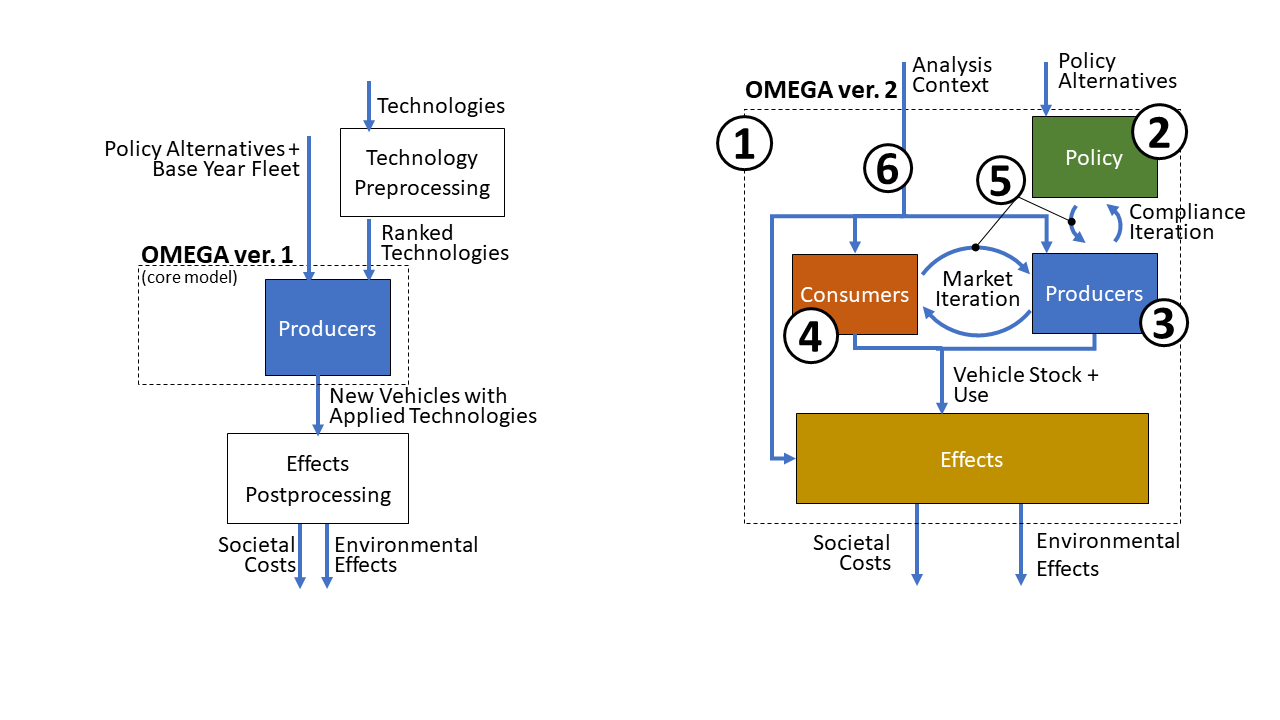
Fig. 1.1 Comparison to prior version of OMEGA
Update #1: Expanded model boundaries. In defining the scope of this model version, we have attempted to simplify the process of conducting a run by incorporating into the model some of the pre- and post-processing steps that had previously been performed manually. At the same time, we recognize that an overly-expansive model boundary can result in requirements for inputs that are difficult to specify. To avoid this, we have set the input boundary only so large as to capture the elements of the system we assume are responsive to policy. This approach helps to ensure that model inputs such as technology costs and emissions rates can be quantified using data for observable, real-world characteristics and phenomena, and in that way enable transparency by allowing the user to maintain the connection to the underlying data. For the assumptions and algorithms within the model boundary, we aim for transparency through well-organized model code and complete documentation.
Update #2: Independent Policy Module. The previous version of OMEGA was designed to analyze a very specific GHG policy structure in which the vehicle attributes and regulatory classes used to determine emissions targets were incorporated into the code throughout the model. In order to make it easier to define and analyze other policy structures, the details regarding how GHG emissions targets are determined and how compliance credits are treated over time are now included in an independent Policy Module and associated policy inputs. This allows the user to incorporate new policy structures without requiring revisions to other code modules. Specifically, the producer decision module no longer contains any details specific to a GHG program structure, and instead functions only on very general program features such as fleet averaging of absolute GHG credits and required technology shares.
Update #3: Modeling of multi-year strategic producer decisions. As a policy analysis tool, OMEGA is intended to model the effect of policies that may extend well into the future, beyond the timeframe of individual product cycles. This version of OMEGA is structured to consider a producer objective function to be optimized over the entire analysis period. Year-by-year compliance decisions account for management of credits which can carry across years in the context of projections for technology cost and market conditions which change over time. The timeframe of a given analysis can be specified anywhere from near-term to long-term, with the length limited only by inputs and assumptions provided by the user.
Update #4: Addition of a consumer response component. The light-duty vehicle market has evolved significantly in the time since the initial release of OMEGA. In particular, as the range of available technologies and services has grown wider, so has the range of possible responses to policy alternatives. The model structure for this version includes a Consumer Module that can be used to project how the light-duty vehicle market would respond to policy-driven changes in new vehicle prices, fuel operating costs, trip fees for ride hailing services, and other consumer-facing elements. The Consumer Module outputs the estimated consumer responses, such as overall vehicle sales and sales shares, as well as vehicle re-registration and use, which together determine the stock of new and used vehicles and the associated allocation of total VMT.
Update #5: Addition of feedback loops for producer decisions. This version of OMEGA is structured around modeling the interactions between vehicle producers responding to a policy and consumers who own and use vehicles affected by the policy. These interactions are bi-directional, in that the producer’s compliance planning and vehicle design decisions will both influence, and be influenced by, the sales and shares of vehicles demanded and the GHG credits assigned under the policy. Iterative feedback loops have now been incorporated; between the Producer and Consumer modules to ensure that modeled vehicles would be accepted by the market at the quantities and prices offered by the producer, and between the Producer and Policy modules to account for the compliance implications of each successive vehicle design and production option considered by the producer.
Update #6: Use of absolute vehicle costs and emissions rates. The previous version of OMEGA modeled the producer application of technologies to a fleet of vehicles that was otherwise held fixed across policy alternatives. With the addition of a consumer response component that models market share shifts, this version utilizes absolute costs and emissions rates to compare vehicle design and purchase decisions across vehicle types and market classes.
1.2. Inputs and Outputs
Like other models, OMEGA relies on the user to specify appropriate inputs and assumptions. Some of these may be provided by direct empirical observations, for example the number of currently registered vehicles. Others might be generated by modeling tools outside of OMEGA, such as physics-based vehicle simulation results produced by EPA’s ALPHA model, or transportation demand forecasts from DOE’s NEMS model. OMEGA has adopted data elements and structures that are generic, wherever possible, so that inputs can be provided from whichever sources the user deems most appropriate.
The inputs and assumptions are categorized according to whether they define the policies under consideration, or define the context within which the analysis occurs.
- Policy alternative inputs describe the standards themselves, including the program elements and methodologies for determining compliance as would be defined for an EPA rule in the Federal Register and Code of Federal Regulations.
- Analysis context inputs and assumptions cover the range of factors that the user assumes are independent of the policy alternatives. The context inputs may include fuel costs, costs and emissions rates for a particular vehicle technology package, attributes of the existing vehicle stock, consumer demand parameters, existing GHG credit balances, producer decision parameters, and many more. The user may project changes in the context inputs over the analysis timeframe based on other sources, but for a given analysis year the context definition requires that these inputs are common across the policy alternatives being compared.
A full description of the input files can be found in Chapter 7.
The primary outputs are the environmental effects, societal costs and benefits, and producer compliance status for a set of policy alternatives within a given analysis context. These outputs are expressed in absolute values, so that incremental effects, costs, and benefits can be evaluated by comparing two policy alternatives for a given analysis context. For example, comparing a No Action scenario to an Action (or Policy) Alternative. Those same policy alternatives can also be compared using other analysis context inputs to evaluate the sensitivity of results to uncertainty in particular assumptions. For example, comparing the incremental effects of a new policy in high fuel price and low fuel price analysis contexts.
1.3. Model Structure and Key Modules
OMEGA has been set up so that primary components of the model are clearly delineated in such a way that changing one component of the model will not require code changes throughout the model. The four main modules — Producer, Consumer, Policy, and Effects — are each defined along the lines of their real-world analogs. Producers and consumers are represented as distinct decision-making agents, which each exist apart from the regulations defined in the Policy Module. Similarly, the effects, both environmental and societal, exist apart from producer and consumer decision-making agents and the policy. This structure allows a user to analyze policy alternatives with consistently defined producer and consumer behavior. It also provides users the option of interchanging any of OMEGA’s default modules with their own, while preserving the consistency and functionality of the larger model.
Producer Module: This module projects the decisions of the regulated entities (producers) in response to policy alternatives, while accounting for consumer demand. The regulated entities can be specified as individual companies, or considered in aggregate as a collection of companies, depending on the assumptions made by the user regarding how GHG credits are averaged or transferred between entities.
Consumer Module: This module projects demand for vehicle sales, ownership and use in response to changes in vehicle characteristics such as price, ownership cost, and other key attributes.
Policy Module: This module determines the compliance status for a producer’s possible fleet of new vehicles based on the characteristics of those vehicles and the policy defined by the user. Policies may be defined as performance-based standards using fleet averaging (for example, determining compliance status by the accounting of fungible GHG credits), as a fixed requirement without averaging (for example, a minimum required share of BEVs), or as a combination of performance-based standards and fixed requirements.
Effects Module: This module projects the physical and cost effects that result from the modeling of producers, consumers, and policy within a given analysis context. Examples of physical effects include the stock and use of registered vehicles, electricity and gasoline consumption, and the GHG and criteria pollutant emissions from tailpipe and upstream sources. Examples of cost effects include vehicle production costs, ownership and operation costs, societal costs associated with GHG and criteria pollutants, and other societal costs associated with vehicle use.
1.4. Iteration and Convergence
OMEGA is intended to find a solution which simultaneously satisfies producer, consumer, and policy requirements while minimizing the producer generalized costs. OMEGA’s Producer and Consumer modules represent distinct decision-making entities, with behaviors defined separately by the user. Without some type of interaction between these modules, the model would likely not arrive at an equilibrium of vehicles supplied and demanded. For example, a compliance solution which only minimizes producer generalized costs without consideration of consumer demand may not satisfy the market requirements at the fleet mix and level of sales preferred by the consumer. Similarly, the interaction between Producer and Policy modules ensures that that with each subsequent iteration, the compliance status for the new vehicle fleet under consideration is correctly accounted for by the producer. Since there is no general analytical solution to this problem of alignment between producers, consumers, and policy which also allows model users to independently define producer and consumer behavior and the policy alternatives, OMEGA uses an iterative search approach.
1.5. Analysis Resolution
The policy response projections generated by OMEGA are centered around the modeled production, ownership, and use of light-duty vehicles. It would not be computationally feasible (nor would it be necessary) to distinguish between the nearly 20 million light-duty vehicles produced for sale each year in the US, and hundreds of millions of vehicles registered for use at any given time. Therefore, OMEGA is designed to operate using ‘vehicles’ which are actually aggregate representations of individual vehicles, while still retaining sufficient detail for modeling producer and consumer decisions, and the policy response. The resolution of vehicles can be set for a given analysis, and will depend on the user’s consideration of factors such as the availability of detailed inputs, the requirements of the analysis, and the priority of reducing model run time.
2. Getting Started
The OMEGA model is written in the open source Python programming language. The model is available in two different packages to suit the particular requirements of the end user:
- For users intending to run the OMEGA model with input modifications only, an executable version is available along with a directory structure and a complete set of sample inputs. This Getting Started chapter is focused on this executable version.
- For users intending to run the OMEGA model with user-definable submodules or other code modifications, a developer version is available in a GitHub repository. For more information on the developer version, please refer to the Developer Guide.
2.1. Downloading OMEGA
Releases of the OMEGA model executable will be available as single .zip files at:
2.2. Installing OMEGA
Create a directory that will be used as the installation directory for the OMEGA model and copy the downloaded .zip file into this directory. Unzip the file into this directory to create the entire OMEGA model file structure.
The folder will contain a readme.txt, the executable, a code folder which contains a copy of the source code, a .pdf of the model documentation, an inputs folder which contains demo batch file(s) and model inputs, and an outputs folder that contains pre-run demo simulations.
2.3. Running OMEGA
The newly created run directory will contain the OMEGA model executable file OMEGA-X.Y.Z-win.exe, where X, Y and Z represent the version number. Opening this file will bring up the OMEGA graphical user interface. The executable takes a few moments to start up, (or it may take longer, depending on the speed of the user’s computer), as it contains compressed data which must be extracted to a temporary folder. A self-contained Python installation is included in the executable and Python does not need to be installed by the user in order to run OMEGA. A console window will also be displayed in addition to the GUI window which shows additional runtime information and any diagnostic messages that may be generated.
The GUI has two file system selection boxes in the Run Model tab; one for choosing the batch file (e.g. ‘test_batch.csv’) and one for choosing the folder where the batch will execute and produce outputs. The output folder for the batch will contain the model source code, the batch file, a log file, a requirements file describing the Python installation details, and subfolders for each simulation session. These session folders will contain an in and an out folder. The in folder contains the complete set of inputs to the session, and the out folder contains the simulation outputs and log file.
2.4. Step by Step Example Model Run
Please refer to the GUI Basics documentation for a step by step execution of the demo example model run.
2.5. Viewing the Results
After OMEGA model runs have completed, the results generated for each session are available in the associated out folder in .csv and .png file formats.
3. Running the Demo Example using the Graphical User Interface (GUI)
3.1. GUI Basics
The EPA OMEGA Model is highly modular and can be run using several methods including but not limited to the command line, the Python environment, and the Graphical User Interface (GUI). The GUI is the best option for new users of OMEGA to reproduce existing model runs and become familiar with the model’s input and output structure. This introduction will guide the user through running the demo example.
After launching the GUI, the ‘Intro’ tab will appear as shown in Fig. 3.1.
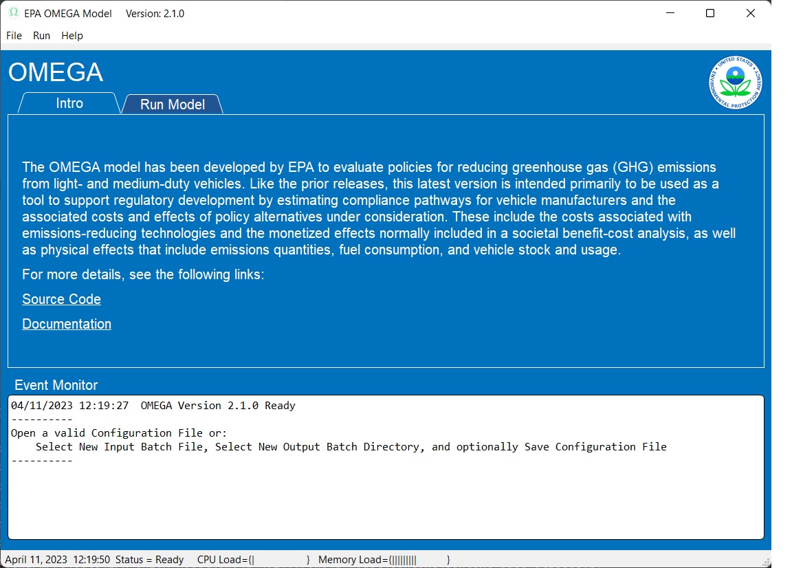
Fig. 3.1 GUI ‘Intro’ Tab
Selecting the ‘Run Model’ tab allows the user to set up an OMEGA model run. The elements of the ‘Run Model’ tab are shown in Fig. 3.2.
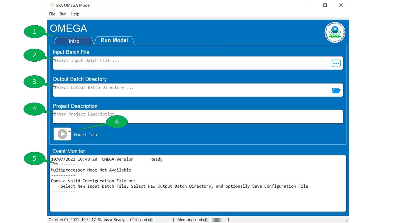
Fig. 3.2 GUI ‘Run Model’ Tab Elements
Description of the ‘Run Model’ tab elements:
Note: Context help is always available by hovering the cursor over an element.
- Element 1 - Tab Selection
- Tabs to select areas of the GUI.
- Element 2 - Input Batch File
- Allows the user to select the Input Batch File. The Input Batch File is a standard OMEGA input file that describes the complete parameters for a model run. The Input Batch File may be selected from the file menu or the “…” button within the element field. When the Input Batch File is selected, the complete path will be displayed. Hovering the cursor over the complete path will display just the base file name.
- Element 3 - Output Batch Directory
- Allows the user to select the Output Batch Directory. The Output Batch Directory instructs OMEGA where to store the results of a model run. The Output Batch Directory may be selected from the file menu or the folder button within the element field. When the Output Batch Directory is selected, the complete path be displayed. Hovering the cursor over the complete path will display just the base file name.
- Element 4 - Project Description
- Allows the user to enter any useful text that will be saved in an optional Configuration File for future reference. This element is free format text to allow standard functions (such as copy and paste) to be used. The saved text will be displayed whenever the Configuration File is opened.
- Element 5 - Event Monitor
- The Event Monitor prompts the user during model run setup (file selection, etc.) and keeps a running record of OMEGA model execution in real time. This is a standard text field to allow simple copying of text as needed for further study or debugging purposes. Log files are also produced in the batch and session output folders as the model runs, in fact the Event Monitor echoes these files as the model runs.
- Element 6 - Run Model
- When everything is properly configured, this button will be enabled for initiation of the OMEGA model run.
3.2. Running the Demo Example
The elements required to run the model are loaded by creating a new model run, or by using an existing Configuration File. As this is the first time the Demo Example will be run, a new model run will be created.
Note: The Event Monitor will provide additional guidance through the model loading process.
3.2.1. Creating a New Model Run From The Demo Example
- Select the ‘Run Model’ tab.
- Load an existing OMEGA Input Batch File using the file menu or button within the field. (Required)
- Select a new or existing OMEGA Output Batch Directory using the file menu or button within the field. (Required)
- Add a Project Description. (Optional)
- Use the file menu to save the new Configuration File. (Optional)
The ‘Run Model’ tab will look similar to Fig. 3.3 below. The displayed values represent one of the supplied demonstration model configurations.
3.2.2. Existing Configuration File
If a model run configuration was previously saved, the configuration may be reloaded to simplify repeating runs. From the file menu, select ‘Open Configuration File’ to launch a standard File Explorer window to load an existing Configuration File. When properly loaded, the ‘Run Model’ tab will look similar to Fig. 3.3 below. The displayed values represent one of the supplied demonstration model configurations.
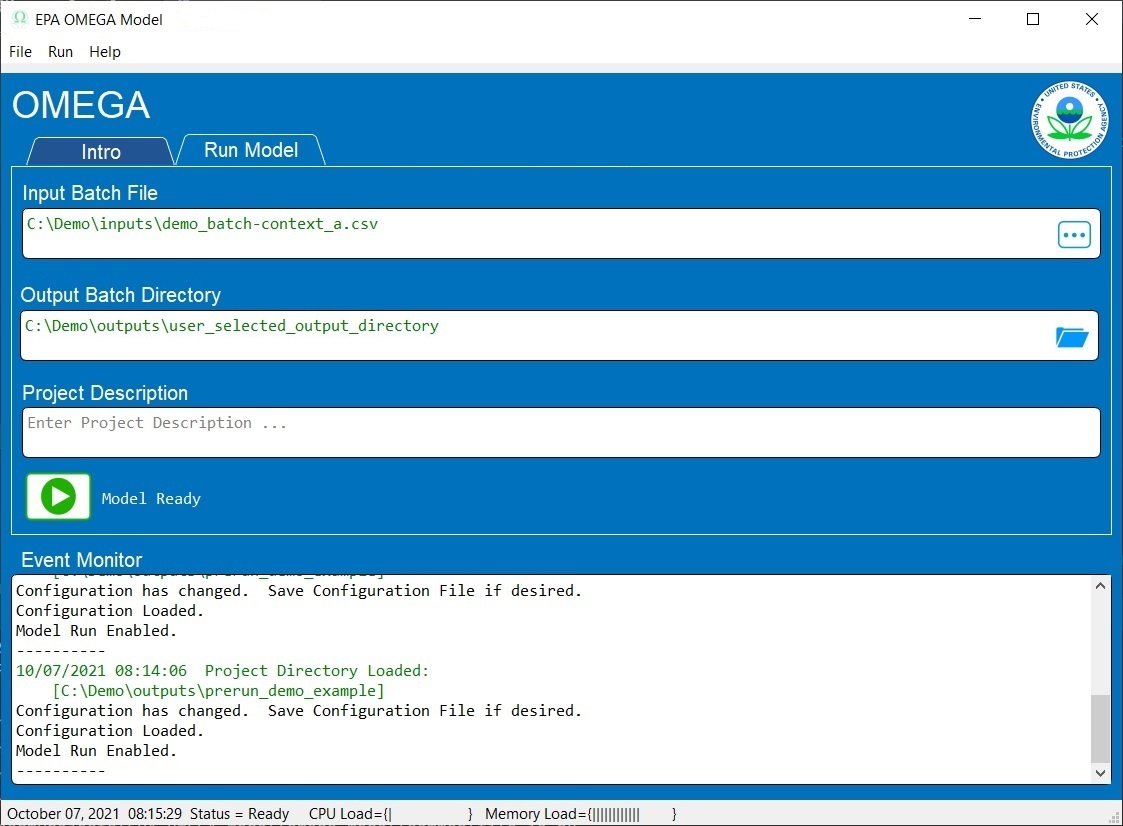
Fig. 3.3 Configuration File Loaded
3.2.3. Running the Model
With all of the model requirements loaded, select the ‘Run Model’ tab and the ‘Model Run’ button will be enabled. Press the ‘Model Run’ button to start the model run.
As the model is running, the ‘Run Model’ tab will look similar to Fig. 3.4 below.
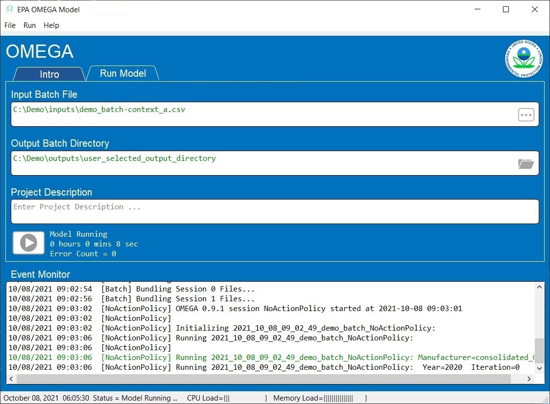
Fig. 3.4 Model Running
The GUI provides real time information during the model run:
- The model starting information is detailed in the event monitor. This includes the time and Input Batch File used.
- The model status, error count, and elapsed time from model start are continuously updated adjacent to the ‘Run Model’ button.
- The load on the system CPU and system Memory is monitored in the Windows Status Bar at the bottom of the GUI window.
- The Event Monitor provides a continuous stream of information gathered from the simultaneous OMEGA processes.
When the model run is completed, the ‘Run Model’ tab will look similar to Fig. 3.5 below.
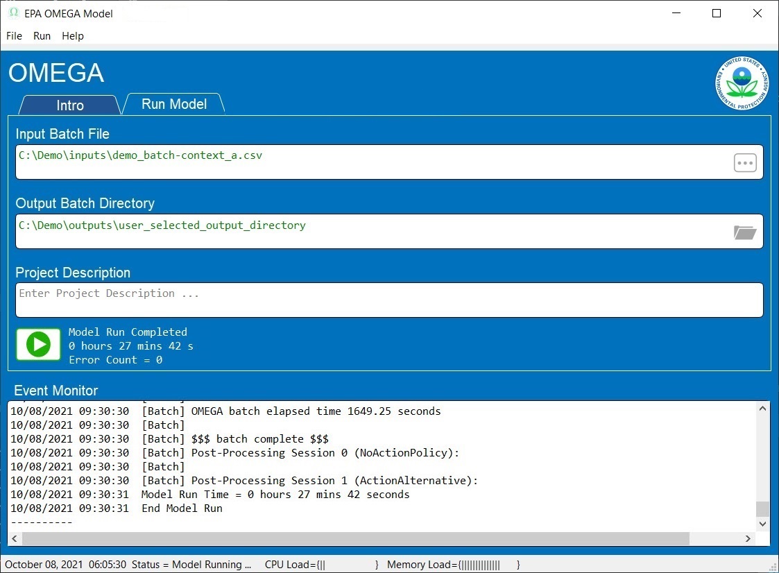
Fig. 3.5 Model Completed
Final GUI Data:
- The model ending information is detailed in the event monitor. This includes the time and the Output Batch Directory used.
- The model status and final model run time are displayed adjacent to the ‘Run Model’ button.
3.3. Interpreting the Demo Example Results
Each session folder has an out folder which contains a number of default outputs. The outputs fall into three categories described in this section: image file outputs, detailed outputs in csv-formatted text files, and a run log text file.
3.3.1. Auto-generated image file outputs
While the detailed modeling results are primarily recorded in csv-formatted text files (described in Table 3.2), OMEGA also produces a number of standard graphical image outputs. This lets the user quickly and easily review the results, without requiring any further post-processing analyses. The various types of auto-generated images are listed in Table 3.1.
| Abbreviated File Name | File Description |
|---|---|
| …Cert Mg v Year…png | compliance including credit transfers, initial and final compliance state |
| …Shares.png | absolute market share by market category, market class, regulatory class and context size class |
| …V Cert CO2e gpmi…png | sales-weighted average vehicle certification CO2e g/mi by market category / class |
| …V Tgt CO2e gpmi…png | sales-weighted average vehicle target CO2e g/mi by market category / class |
| …V kWh pmi…png | sales-weighted average vehicle cert direct kWh/mi by market category / class |
| …V GenCost…png | sales-weighted average vehicle producer generalized cost by market category / class |
| …V Mg…png | sales-weighted average vehicle cert CO2e Mg by market category / class |
| …Stock CO2 Mg.png | vehicle stock CO2 emissions aggregated by calendar year |
| …Stock Count.png | vehicle stock registered count aggregated by calendar year |
| …Stock Gas Gallons.png | vehicle stock fuel consumed (gasoline gallons) aggregated by calendar year |
| …Stock kWh.png | vehicle stock fuel consumed (kWh) aggregated by calendar year |
| …Stock VMT.png | vehicle stock distance travelled (miles) aggregated by calendar year |
Demo example: Reading the manufacturer compliance plot
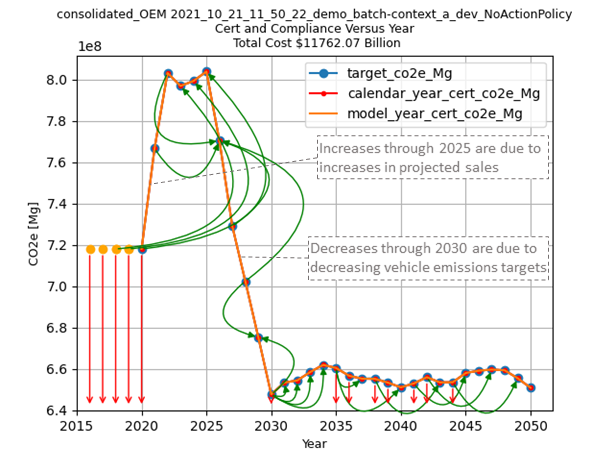
The manufacturer compliance plot provides several visual details on how the manufacturers are achieving compliance (or not) for each model year, and is a good starting point to inform the user of the model results. An example run with the demo inputs is shown in Fig. 3.6.
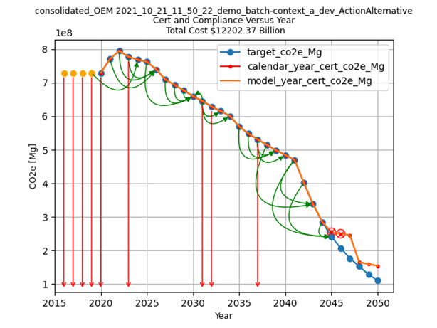
Fig. 3.6 Typical manufacturer compliance plot
The following describes the key features of this plot:
- The Y-axis represents the total CO2e emissions, in metric tons (or Mg) for each model year.
- The blue line and dots represent the required industry standard for each year, in metric tons (Mg).
- The orange line represents the industry-achieved net standard after credits have been applied or carried to other model years. The orange dots represent the existence of credits banked prior to the analysis start year (they are placed on the chart to be visible, but the Mg level of the dots has no meaning.)
- Green arrows indicate the source model year (arrow origin) and the model year in which credits have been applied (arrow end.)
- Vertical down arrows, in red, indicate that some or all of the credits generated by that model year expired unused.
- Red circle-x symbols indicate years that compliance was not achieved, after considering the carry-forward and carry-back of credits.
Demo example: Using image files to compare policy alternative results for Context A
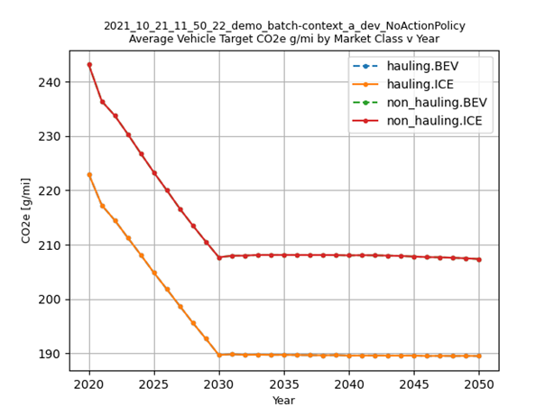
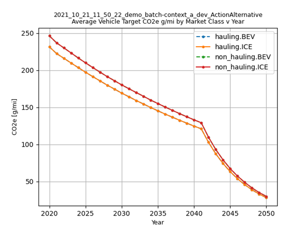
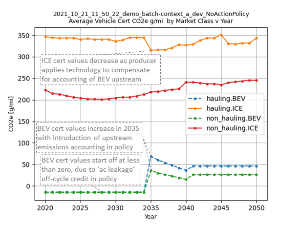
In this demo example, the action alternative (Alt 1) is generally more stringent than the no-action alternative (Alt 0), so we should expect to see this difference in policy reflected in the results. Fig. 3.7 highlights some of the main differences between these two alternatives. The upper panels show the GHG targets (grams CO2e per mile), which decrease in each model year through 2030 in Alt 0, while in Alt 1 the targets are decreasing through 2050 with an accelerated rate after 2041. While the GHG targets are determined at the vehicle level, the plots shown here are weighted average values for each market class. The underlying individual vehicle targets are available in the ‘…vehicles.csv’ output file (see Table 3.2) and are a function of the respective policy definitions and the attributes of the vehicles that are used in the assignment of targets. See Section 4.2 and Table 4.4 for more detail on the policy definitions. For both policy alternatives, the targets are lower for vehicles in the non-hauling market category compared to hauling. Note that there is no difference in the targets between BEV and ICE vehicles within the hauling and non-hauling market categories.
The lower panels show the certification emissions, which like the targets, are also expressed here in CO2e grams per mile. These values are the result of producer, consumer, and policy elements in the model run. For the less stringent Alt 0, the ICE market classes show some modest reduction in certification emissions in the earlier years, which then level off and begin increasing after 2035. For BEVs, certification levels actually begin with negative values due to the policy application of off-cycle credits; specifically, ‘ac leakage’ technology, as defined in the ‘offcycle_credits…csv’ input files. In Alt 0, upstream emissions are applied to BEV certification values beginning in 2035. The no-action policy upstream emissions rates (defined in ‘policy_fuels-alt0.csv’) decline from 2035 to 2040, as reflected in the declining BEV certification emissions over that timeframe. For the more stringent Alt 1, ICE certification values decrease nearly through 2050. In 2045, the available ICE technologies have been exhausted, and certification values level off at the minimum possible levels. BEV certification levels remain constant throughout for Alt 1, and reflect only off-cycle credits since there is no accounting for upstream emissions in this policy alternative.
 |
 |
 |
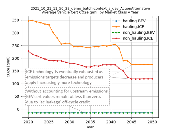 |

Fig. 3.7 Target CO2 (upper) and certification CO2 (lower) for no-action (left, Alt 0) and action (right, Alt 1) policy alternatives
Fig. 3.8 shows the compliance results for the two policy alternatives used in this demo example. The year-to-year changes in targets (blue points) reflect the CO2e grams per mile targets shown in Fig. 3.7, as well as changes in sales and other policy elements used to calculate and scale the absolute Mg CO2e values, such as multipliers and VMT. Certification emissions (red points) generally overlay the targets in each year. Similarly, compliance emissions (orange line) are aligned with certification emissions, since the strategic use of existing credits has not been implemented in the model for this demo. Minor corrections for year-over-year credit transfers are shown with the green arrows, although the magnitude of transfers is small for this demo; larger transfers would be discernible as a difference between the red points and orange line. For Alt 1, the certification emissions begin to depart from the targets in 2045. With insufficient credits to carry-forward (or carry-back) to 2045 and 2046, those two years are non-compliant (red circle-x symbols.) The remaining years, 2047-2050, have an indeterminate compliance status since the demo example was only run out to 2050, and there is still a possible opportunity to carry-back credits from future years.
 |
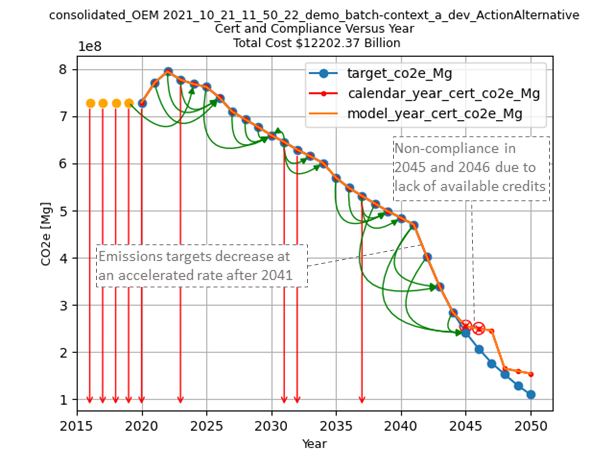 |
Fig. 3.8 Compliance results for no-action (left, Alt 0) and action (right, Alt 1) policy alternatives
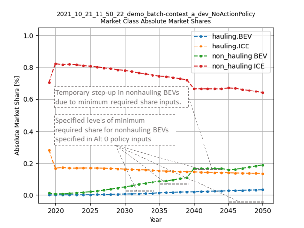
Fig. 3.9 shows new vehicle shares by market class. The more stringent Alt 1 has higher BEV shares for both hauling and non-hauling market classes compared to the less stringent Alt 0. The significant increase in BEV shares in 2048 coincides with the producer’s state of non-compliance; the producer’s attempts to maximize BEV share at this time is limited by the consumer share response (defined in ‘sales_share_params-cntxt_a.csv’), and the specified limits on producer price cross-subsidization (defined in ‘demo_batch-context_a.csv’.) BEV shares also increase in the less stringent Alt 0, although at a slower rate than the action alternative. This increase occurs smoothly as BEVs become relatively less expensive due to cost learning over time. A step-up and plateau in BEV shares from 2040 to 2044 is due to the no-action policy’s minimum production requirement values, specified in ‘required_sales_share-alt0.csv’.
 |
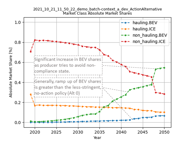 |
Fig. 3.9 Market class shares for no-action (left, Alt 0) and action (right, Alt 1) policy alternatives
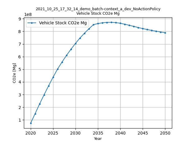
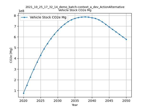
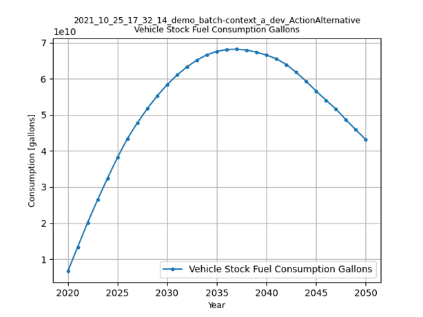
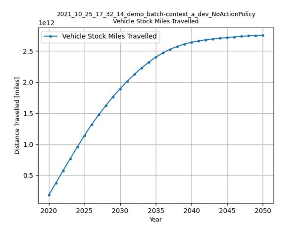
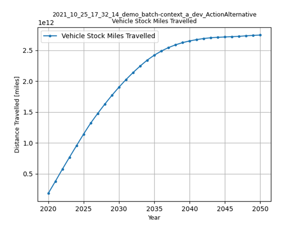
Fig. 3.10 shows some of the key results for the overall vehicle stock. For this example, the base year vehicle inputs (specified in ‘vehicles.csv’) do not contain any information about any vehicles older than age 0 (i.e. MY 2019) in the base year. Therefore, the growth trend that is exhibited in all the panels of Fig. 3.10 is a function of the increasing stock of vehicles that are accounted for as the model progresses over the analysis years. If the model were run with additional data for older vehicles in the base year inputs, the curves shown in these results would appear flatter. When comparing policy alternatives, it is the incremental changes that will likely be of most interest to the user. That information can be gathered from the csv-formatted output files, as described in Table 3.2. These auto-generated image files are mainly intended to provide a high-level view of the key results.
In the first row of Fig. 3.10, the CO2e emissions results from the Effects Module are shown for the two policy alternatives. While the order of magnitude is similar to the Mg CO2e shown in the compliance plot in Fig. 3.8, there are some important differences. First, Fig. 3.10 shows the combined effects for the entire on-road stock, rather than the effects of only new vehicles. Second, the VMT assumptions used for Fig. 3.10 are meant to represent the on-road usage, as a function of vehicle age, while the Mg CO2e values for the compliance plot are based on policy-defined lifetime VMT. Finally, the Mg CO2e values in Fig. 3.10 include all CO2e emissions, direct (tailpipe) and indirect (upstream), while the interpretation of Mg CO2e in the compliance plot may vary year-to-year depending on whether the policy includes consideration of upstream emissions or not.
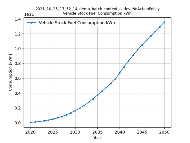
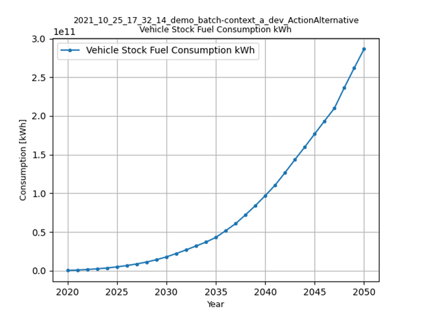
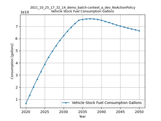
The second row of Fig. 3.10 shows the kWh consumed for the no-action policy (Alt 0) and the action alternative (Alt 1.) Note the difference in scale; Alt 1 electricity consumption in 2050 is more than two times Alt 0 due to the higher penetration of BEVs in the vehicle stock. Partly because of this increase in BEVs (in addition to technology added to ICE vehicles), the third row of Fig. 3.10 shows gasoline consumption tapering off more dramatically for Alt 1 by 2050.
The fourth row of Fig. 3.10 shows total vehicle miles traveled (VMT) for the vehicle stock. There is no endogenous response for per-vehicle VMT included in this demo example (e.g. the VMT rebound effect), so the curves here show only minor VMT differences between policy alternatives due to the differences in overall sales.
The final row of Fig. 3.10 shows the total registered count of vehicles for each year which indicates the effect of adding new vehicles (the rate of increase in the early years) and the effect of de-registering vehicles (the rate of increase slows in later years as the de-registration rate approaches the re-registration rate).
 |
 |
 |
 |
 |
 |
 |
 |
 |
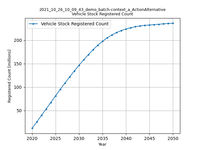 |
Fig. 3.10 MY2020+ vehicle stock GHG emissions (1st row), kWh consumption (2nd row), gasoline consumption (3rd row), VMT (4th row) and registered count (5th row) for no-action (left, Alt 0) and action (right, Alt 1) policy alternatives
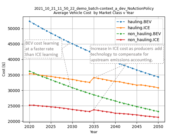
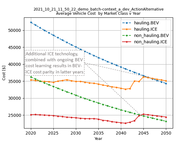
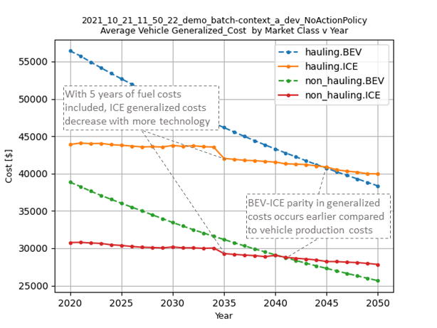
Fig. 3.11 shows the vehicle production costs (upper panels) and producer generalized costs (lower panels) for the two policy alternatives. BEV production costs decrease at a faster rate than ICE vehicles due to cost learning (as defined in the ‘simulated_vehicles.csv’ inputs.) Still, in the less stringent no-action policy (Alt 0) BEV production costs remain higher than ICE costs throughout the analysis timeframe. That’s not true for the more stringent action alternative (Alt 1), where production cost parity is reached in 2045 as additional technology added causes ICE costs to converge with BEV costs. The lower panels of Fig. 3.11 show that producer generalized costs follow the same trends as vehicle production costs. However, there are a few important differences; First, the generalized costs in this example include the portion of fuel cost that producers assume is valued by consumers in the purchase decision (defined in ‘producer_generalized_cost.csv’), making generalized costs higher than production costs. Note that the increase in Alt 0 ICE production costs in 2035 actually corresponds to a decrease in generalized costs, as the addition of ICE technology changes the fuel consumption rates, and therefore the fuel operating costs per mile. Second, because of the difference in fuel operating costs for BEV and ICE vehicles, cost parity occurs earlier for generalized costs than for production costs.
 |
 |
 |
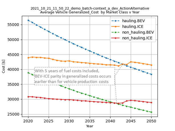 |
Fig. 3.11 Vehicle Production Cost (upper) and Generalized Cost (lower) for no-action (left, Alt 0) and action (right, Alt 1) policy alternatives
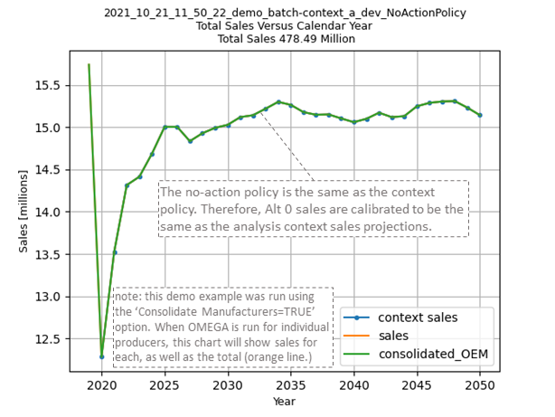
In this demo example, overall new vehicle sales are determined by the assumed price elasticity of demand (-1, as defined in ‘demo_batch-context_a’.csv’), and the change in generalized cost for vehicles relative to the analysis context. Fig. 3.12 shows the sales results for the two policy alternatives. Because the no-action alternative (left panel) is the same as the context policy, the model automatically calibrates the aggregate generalized cost in each year so that overall sales volumes match the analysis context sales projections. See Section 4.4 for more details. The right panel shows sales for the action alternative, Alt 1. Deviations from the projected sales, above and below, are the result of differences in generalized costs between the two alternatives. Prior to 2035, Alt 1 has lower generalized costs then Alt 0, so sales are higher than the context projections. After 2035, Alt 1 has higher generalized costs, so sales are lower than the context projections. Fig. 3.14 shows the incremental generalized costs as derived from the ‘…summary_results.csv’ output file.
 |
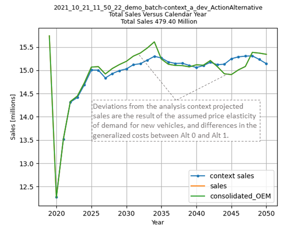 |
Fig. 3.12 Total new vehicle sales for no-action (left, Alt 0) and action (right, Alt 1) policy alternatives
3.3.2. Detailed csv-formatted text output files
While the auto-generated image files are convenient for quickly looking at high-level results, the csv-formatted output files provide a full accounting of detailed results. This includes the full range of modeled effects, both physical and monetary, as well as credit logs to provide a better understanding of producer compliance decisions, and intermediate iteration steps to help illuminate the producer-consumer modeling. The resolution of the majority of these output files is at the same level defined by the user in the run inputs; namely by producer, vehicle, and analysis year. Table 3.2 summarizes the complete set of csv-formatted output files.
| Abbreviated File Name | File Description |
|---|---|
| …summary_results.csv | contains the data from the image files |
| …GHG_credit_balances.csv | beginning and ending model year GHG credit balances by calendar year |
| …GHG_credit_transactions.csv | model year GHG credit transactions by calendar year |
| …manufacturer_annual_data.csv | manufacturer compliance and cost data by model year |
| …vehicle_annual_data.csv | registered count and VMT data by model year and age |
| …vehicles.csv | detailed base year and compliance (produced) vehicle data |
| …new_vehicle_prices.csv | new vehicle sales-weighted average manufacturer generalized cost data by model year |
| …producer_consumer_iteration_log.csv | detailed producer-consumer cross-subsidy iteration data by model year |
| …cost_effects.csv | vehicle-level cost effects data by model year and age |
| …physical_effects.csv | vehicle-level physical effects data by model year and age |
| …tech_tracking.csv | vehicle-level technology tracking data by model year and age |
Four of these output files, in particular, may be helpful for the user to better understand the details of the model results; ‘summary_results.csv’, ‘physical_effects.csv’, ‘cost_effects.csv’, and ‘tech_tracking.csv.’ The examples given here are meant to illustrate how these outputs can be used to quantify specific effects of the policies. A full description of the fields contained the csv output files is provided in Chapter 7.
Summary results output file
The ‘summary_results.csv’ output file is unique among the csv-formatted output files in that it combines results for all sessions in a batch into a single file. While some of the other output files contain significantly more detail and vehicle-level resolution, the summary file is a convenient source for some of the important key outputs, and is aggregated to a single row for each session + analysis year.
Demo example: Using the ‘summary_results.csv’ file to compare policy alternative results for Context A
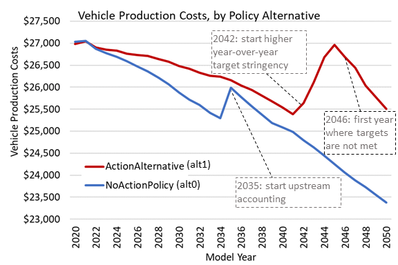
Fig. 3.13 shows vehicle production costs for the action (Alt 1) and no-action (Alt 0) policy alternatives. These values are the same as those shown in the auto-generated images in Fig. 3.11, combined into a single plot. In the right panel, the incremental costs have been calculated from the ‘summary_results.csv’ file. The most impactful effects of the policy definitions can be seen here: in 2035, the incremental cost of Alt 1 is reduced as upstream emissions accounting is introduced in the no-action case; in 2042, the incremental cost begins to increase as the Alt 1 year-over-year stringency increases.
 |
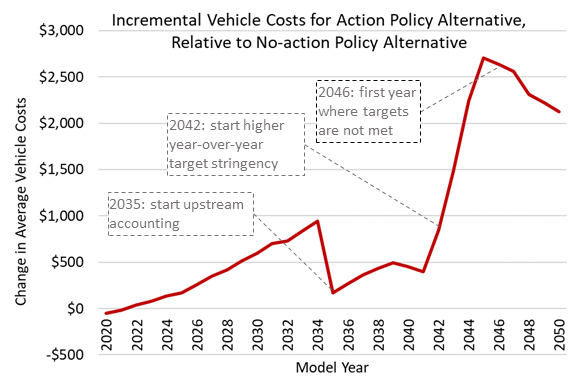 |
Fig. 3.13 Average per vehicle production cost: absolute costs (left), and change in costs due to the action alternative policy (right)
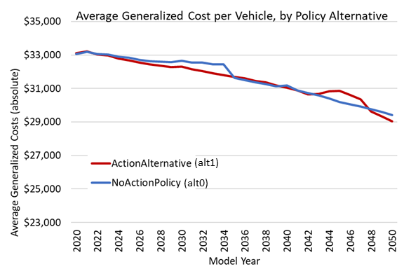
Fig. 3.14 shows the producer generalized costs for the action and no-action policy alternatives. As with the auto-generated image files showing generalized costs, the costs here are higher than vehicle production costs because of the example’s inclusion of 5 years of fuel operating costs. The incremental generalized costs shown in the right panel are helpful for understanding the sales effects shown in Figure Fig. 3.12. In the years when the action alternative has higher generalized costs, new vehicles sales decrease relative to the analysis context projections; and when costs are lower, new vehicle sales are higher.
 |
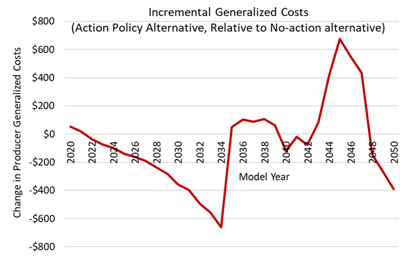 |
Fig. 3.14 Vehicle generalized cost: absolute costs (left), and change in costs due to the action alternative policy (right)
Physical effects output file
The ‘physical_effects.csv’ file provides details such as the quantity of GHG and criteria pollutants, fuel consumption, number of registered vehicles, and vehicle miles traveled. These data are presented at the vehicle level for all model years and ages included in the model run. For any given calendar year, the associated rows in the file represent the effects associated with the stock of registered vehicles at that time, considering new vehicles that have been sold and existing vehicles that have been re-registered. The units of each data field in the file are included in the header (i.e., the field name) for each column of data. With this file, the user can explore physical effects by vehicle ID, model year, age, calendar year, manufacturer, regulatory class, in-use fuel, or market class.
Demo example: Using the ‘physical_effects.csv’ file to compare policy alternative results for Context A
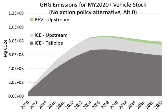
Fig. 3.15 shows the CO2e emissions of the action alternative (Alt 1) and the no-action policy alternative (Alt 0.) The total values are the same as in the auto-generated image outputs shown in Fig. 3.10. The csv-formatted outputs shown here allow both alternatives to be shown with a breakdown by direct (tailpipe) and indirect (upstream) emissions. The contribution of BEV upstream emissions is lower in the left panel because of the lower BEV shares for Alt 0, compared to the more stringent Alt 1 policy in the right panel. In contrast, ICE emissions (both tailpipe and upstream) taper off more in the latter years for Alt 1 due to the combination of fewer ICE vehicles in use, and greater application of technologies which reduce fuel consumption and emissions.
 |
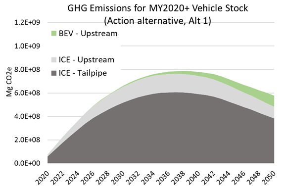 |
Fig. 3.15 GHG emissions with upstream and tailpipe breakdown for no-action (left, Alt 0) and action (right, Alt 1) policy alternatives
Technology tracking output file
Demo example: Using the ‘tech_tracking.csv’ file to compare policy alternative results for Context A
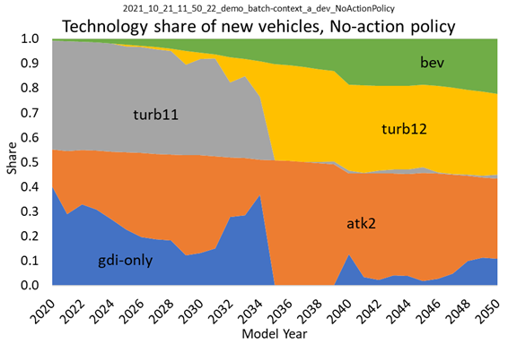
Fig. 3.16 shows the shares of applied technologies at the level of resolution specified by the tech package details in the ‘simulated_vehicles.csv’ input file. While the particular details of the technology package definitions are not relevant for the purpose of this example, the differences between policy alternatives is illustrative. With the more stringent action alternative (Alt 1), BEV shares are clearly higher than in Alt 0, especially in the years approaching 2050. The technology packages with ‘turb12’ and ‘atk2’ have lower certification emissions than the packages with ‘turb11’ and ‘gdi-only’, so the transition to the more advanced packages occurs earlier in the analysis timeframe under the more stringent Alt 1, accordingly.
 |
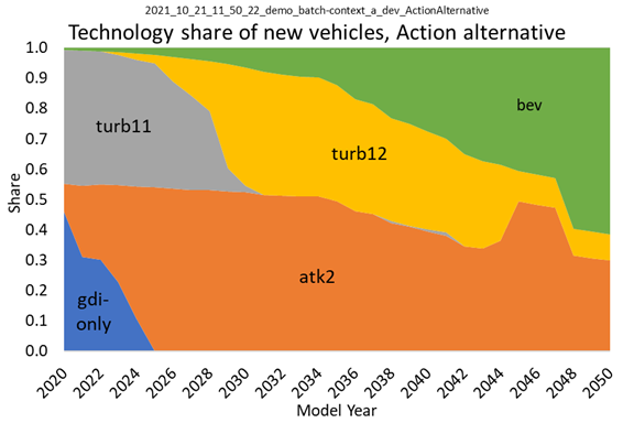 |
Fig. 3.16 Technology shares for no-action (left, Alt 0) and action (right, Alt 1) policy alternatives
Cost effects output file
The ‘cost_effects.csv’ file provides all of the monetized effects associated with the physical effects described above. Like the physical effects, the monetized costs are reported on an absolute basis. However, since the user will likely be most interested in the difference in costs between two policy alternatives, it is left up to the user to take advantage of the csv-formatted outputs to calculate the values that are most useful.
Demo example: Using the ‘cost_effects.csv’ file to compare policy alternative results for Context A
Fig. 3.17 shows the cost elements that would be used in a societal benefits-cost analysis. The dark orange curve represents the net costs as the sum of costs for technology, GHG pollution, fuel, noise, energy security, criteria pollutants, and congestion. In the earlier years, the net costs are positive, and then changing to negative (i.e. benefits) after 2031. This tendency is due to the accounting convention used within the Effects Module, where the costs for technologies are counted at the time a new vehicle is produced, while the fuel consumption and emissions (and associated costs) accrue over the lifetime of a vehicle. This delayed response due to the turnover and use of the vehicle stock is especially evident in 2035; at this point, the incremental technology costs are dramatically reduced as the no-action alternative becomes effectively more stringent with the introduction of upstream accounting. However, the impacts on other costs (fuel, emissions, etc.) show up more gradually as the vehicle stock continually turns over with new vehicles.
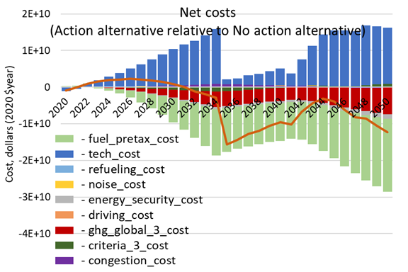
Fig. 3.17 Net cost, with breakdown of contributing costs, for the action alternative relative to the no-action policy
3.3.3. Run log output file
| Abbreviated File Name | File Description |
|---|---|
| o2log…txt | session console output |
The session log file contains console output and may provide useful information in the event of a runtime error.
Post-processing Notes
Post-compliance-modeling image files and other outputs are generated by omega_model.postproc_session.
The producer-consumer iteration log and new vehicle price files as well as the log file are generated and/or saved during compliance modeling rather than post-processing.
4. Model Architecture and Algorithms
OMEGA is structured around four main modules which represent the distinct and interrelated decision-making agents and system elements that are most important for modeling how policy influences the environmental and other effects of the light duty sector. This chapter begins with a description of the simulation process, including the overall flow of an OMEGA run, and fundamental data structures and model inputs. That section is followed by descriptions of the algorithms and internal logic of the Policy Module, Producer Module, and Consumer Module, and then by a section on the approach for Iteration and Convergence Algorithms between these three modules. Finally, the accounting method is described for the physical and monetary effects in the Effects Module.
Throughout this chapter, references to a demo analysis are included to provide additional specificity to the explanations in the main text. These examples, highlighted in shaded boxes, are also included with the model code. Please refer to Section 3.2.3 for more information on how to view and rerun the demo analysis.
4.1. Overall Simulation Process
4.1.1. Simulation Scope and Resolution
The model boundary of OMEGA as illustrated in Fig. 4.1 defines the system elements which are modeled internally, and the elements which are specified as user inputs and assumptions. The timeframe of a given analysis spans the years between analysis start and end years defined by the user. Together, the boundary and analysis timeframe define the scope of an analysis.
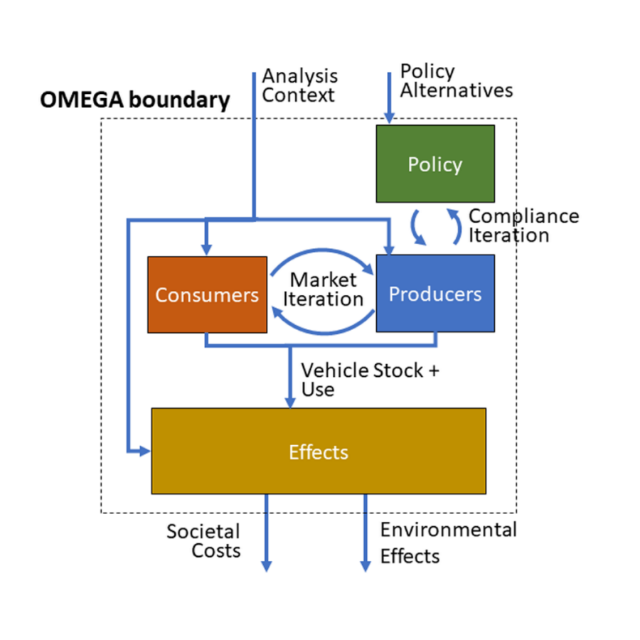
Fig. 4.1 OMEGA model boundary
Demo example: Analysis timeframe
For the demo analysis, the base year is defined as calendar year 2019. The year immediately following the base year is automatically used as the analysis start year. The analysis final year in this example is set to 2050 in the ‘demo_batch-context-X.csv’ input file. Therefore, the analysis timeframe is a 31-year span, inclusive of 2020 and 2050. The selection of 2019 as the base year is automatically derived from the last year of historical data contained in the ‘vehicles.csv’ and ‘ghg_credits.csv’ input files. These inputs describe the key attributes and counts for registered vehicles, and producers’ banked Mg CO2e credits as they actually existed. Note that for this example, base year vehicle inputs are limited to MY2019 new vehicles and their attributes. For an analysis which is intended to project the impacts of various policy alternatives on the reregistration and use of earlier model years, the base year inputs would describe the entire stock of registered vehicles, including MY2018, MY2017, etc.
Typically, the analysis start year will already be in the past at the time the model is run. Having the most up-to-date base year data can reduce the number of historical years that need to be modeled, although as noted in the sidebar, there are usually limits to data availability. Some overlap between the modeled and historical years may be beneficial, as it gives the user an opportunity to validate key model outputs against actual data and adjust modeling assumptions if needed.
Model inputs for the policy alternatives and analysis context projections must be available for every year throughout the analysis timeframe. Many of the input files for OMEGA, utilize a ‘start_year’ field, which allows the user to skip years with repetitive inputs if desired. In general, OMEGA will carry over input assumptions from the most recent prior value whenever the user has not specified a unique value for the given analysis year. Similarly, in cases where the user-provided input projections do not extend to the analysis end year, the value in the last specified year is assumed to hold constant in subsequent years. For example, in the demo analysis, 2045 is the last year for which input values are specified in ‘cost_factors-criteria.csv’, so OMEGA will apply the same 2045 values for 2046 through 2050.
An OMEGA analysis can be conducted at various levels of resolution depending on the user’s choice of inputs and run settings. The key modeling elements where resolution is an important consideration include vehicles, technologies, market classes, producers, and consumers.
Vehicle resolution: The definition of a ‘vehicle’ in an OMEGA analysis is an important user decision that determines one of the fundamental units of analysis around which the model operates. In reality, the vehicle stock is made up of hundreds of millions of vehicles, owned and operated by a similarly large number of individuals and companies. Theoretically, a user could define the vehicle resolution down to the individual options and features applied, or even VIN-level of detail. But given limitations in computational resources, the OMEGA user will more likely define vehicles at the class or nameplate level (e.g. ‘crossover utility vehicle’, or ‘AMC Gremlin’.) Regardless of how vehicles are represented, OMEGA will retain the details of each vehicle throughout the model (including in the outputs) at the level of resolution that the user has chosen. For example, if a user defines vehicle inputs at the nameplate level, the outputs will report nameplate level vehicle counts, key attributes, emissions rates, and physical and cost effects.
Technology package resolution: In OMEGA, producer decisions are made using complete packages of technologies which are integral to, and inseparable from, the definition of a candidate vehicle. In other words, a change to any of the individual technology components would result in a different candidate vehicle. The ‘simulated_vehicles.csv’ file contains the information for each candidate vehicle that is needed for modeling producer decisions, including the costs and emissions rates that are associated with the technology package.
Technology component resolution: Though the model operates using full technology packages (mentioned above), it may sometimes be helpful to track the application of particular sub-components of a package. The user can choose to add flags to the ‘simulated_vehicles.csv’ file to identify which types of components are present on the candidate vehicles. These flags are then used by the model to tabulate the penetration of components in the vehicle stock over time.
Market class resolution: The level of detail, and type of information used within the Producer and Consumer modules is different. For example, we assume that consumers are not aware of the compliance implications and detailed design choices made by the producer, unless those factors are evident in the price, availability, or key attributes of a vehicle. Therefore, consumer decisions regarding the demanded shares of vehicles are modeled based on vehicle characteristics aggregated at the market class level. The user’s determination of the appropriate resolution for the market classes will depend on the chosen specification for share response modeling within the Consumer Module. Note that within the Consumer Module, while share response is modeled at the market class level, other consumer decisions (like reregistration and use) can be based on more detailed vehicle-level information.
Producer resolution: The producers in OMEGA are the regulated entities subject to the policy alternatives being analyzed and are responsible (together with the consumers and policy) for the decisions about the quantities and characteristics of the vehicles produced. The user can choose to model the producers either as an aggregate entity with the assumption that compliance credits are available in an unrestricted market (i.e. ‘perfect trading’), or as individual entities with no trading between firms.
Consumer resolution: The approach to account for heterogeneity in consumers is an important consideration when modeling the interaction between producer decisions and the demand for vehicles. By taking advantage of user-definable submodules, a developer can set-up the Consumer Module to account for different responses between consumer segments.
Whatever the level of resolution, the detail provided in the inputs 1) must meet the requirements of the various modeling subtasks, and 2) will determine the level of detail of the outputs. When preparing analysis inputs, it is therefore necessary to consider the appropriate resolution for each module. For example:
- Within the Policy Module, vehicle details are needed to calculate the target and achieved compliance emissions. This might include information about regulatory classification and any vehicle attributes that are used to define a GHG standard.
- Within the Producer Module, the modeling of producer decisions requires sufficient detail to choose between compliance options based the GHG credits and generalized producer cost associated with each option.
- Within the Consumer Module, the modeling of consumer decisions requires sufficient detail to distinguish between market classes for representing both the purchase choices among different classes, and the reregistration and use of vehicles within a given class.
Demo example: Modeling resolution
| Modeling element | Where is the resolution defined? | Description of resolution in the demo |
|---|---|---|
| Vehicle resolution | vehicles.csv | 51 2019 base year vehicles differentiated by context size class (‘Small Crossover’ ‘Large Pickup’ etc) manufacturer_id and electrification_class (‘N’ ‘HEV’ ‘EV’) |
| Technology package resolution: | simulated_vehicles.csv | 578088 candidate vehicles for the analysis timeframe 2020 through 2050 with technology packages for ICE and BEV powertrains |
| Technology component resolution: | simulated_vehicles.csv | detailed flags for identifying technology package contents of ac_leakage ac_efficiency high_eff_alternator start_stop hev phev bev weight_reduction deac_pd deac_fc cegr atk2 gdi turb12 turb11 |
| Market class resolution | consumer.market_classes.py user-definable submodule and market_classes.csv | 4 classes in 2 nested levels with BEV and ICE categories within first tier hauling and non-hauling categories |
| Consumer resolution | consumer.sales_share_gcam.py user-definable submodule | consumer heterogeneity is inherent in share weights used to estimate market class shares |
| Producer resolution | demo_batch-context-X.csv and manufacturers.csv | 2 producers (‘OEM_A’ and ‘OEM_B’) and ‘Consolidate Manufacturers’ run setting set to FALSE |
4.1.2. Process Flow Summary
In an OMEGA session, the model runs by looping over analysis years and producers. Within each successive loop, the simulation of producer and consumer decisions results in new vehicles entering the stock of registered vehicles, and the reregistration and use of existing vehicles from the prior year’s stock.
As shown in Fig. 4.2 , this simulation process involves two iterative loops. In one loop, the Policy Module determines whether or not the producer’s strategic compliance target is met by the candidate production options under consideration. In the other iterative loop, the Consumer Module determines whether or not the market will accept the quantities of vehicles offered at the prices set by the producer. Both the Producer-Policy and the Producer-Consumer iterative loops must achieve convergence for the simulation to proceed. Once all the analysis years and producers have been completed, the effects calculations are performed and results are written to the output files.
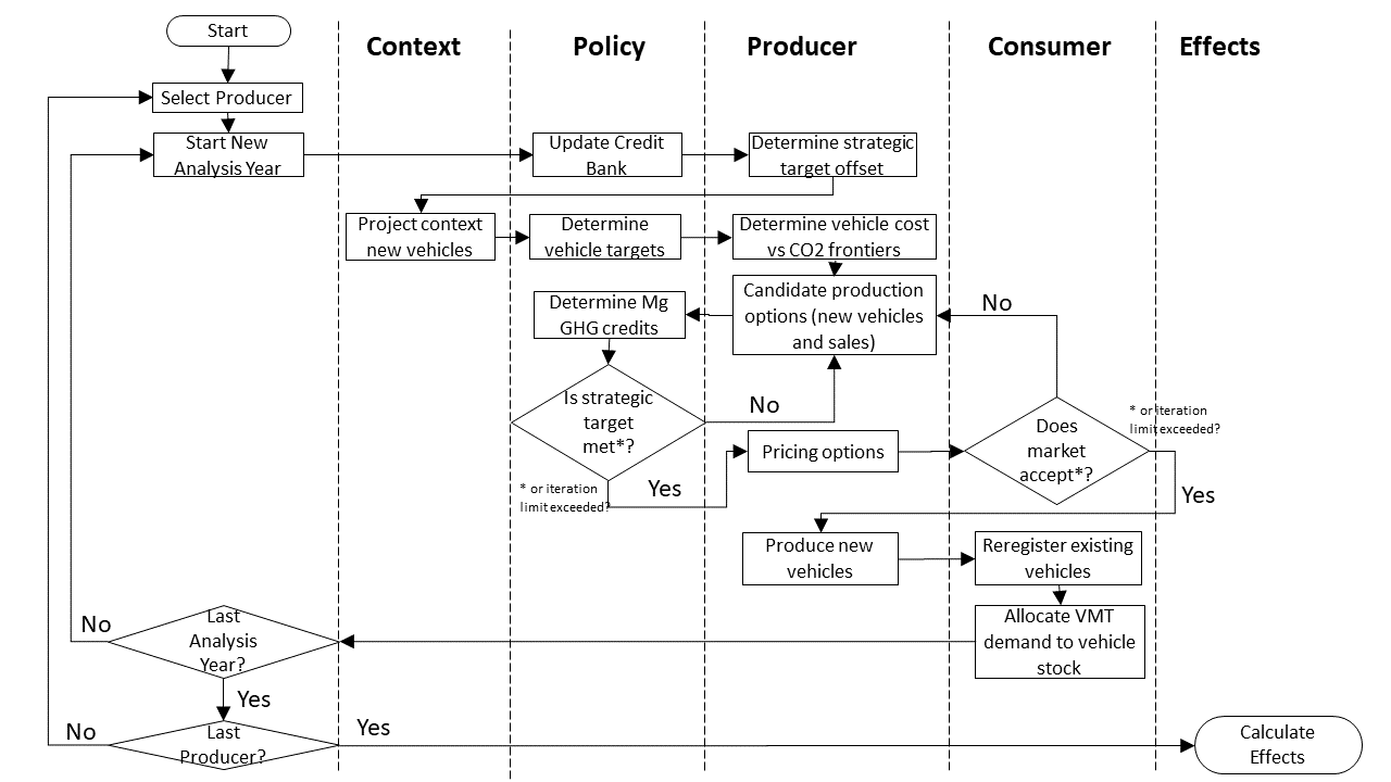
Fig. 4.2 OMEGA process flow
4.1.3. Model Inputs
As described in the Section 1.2 overview, OMEGA model inputs are grouped into two categories; policy alternative inputs and analysis context inputs. The policy alternatives define the GHG standards that are being evaluated by the model run, while the analysis context refers collectively to the external assumptions that apply to all policies under analysis.
Policy Alternatives Inputs
An OMEGA run requires a full description of the GHG standards themselves so that the modeled producer compliance considerations are consistent with how an EPA rule would be defined in the Federal Register and Code of Federal Regulations. As described in Section 4.2, OMEGA is intended primarily for the analysis of fleet averaging standards, and the demo example has been set up to illustrate how accounting rules for GHG credits in a fleet averaging program can be defined. This includes the coefficients for calculating emissions rate targets (gram CO2e per mile) based on vehicle attributes, the methods for determining emissions rate certification values (e.g. drive cycle and fuel definitions, off-cycle credits), and the rules for calculating and accounting for Mg CO2e credits over time (e.g. banking and trading rules, and lifetime VMT assumptions.) See Table 4.4 for a complete list of the policy alternative inputs used in the demo example.
Analysis Context Inputs
The analysis context defines the inputs and assumptions that the user assumes are independent of the policy alternatives. This clear delineation of exogenous factors is what enables the apples-to-apples comparison of policy alternatives within a given analysis context. This is the primary purpose for which OMEGA was designed – to quantify the incremental effects of a policy for informing policy decisions. At the same time, considering how the incremental effects of a policy might vary depending on the analysis context assumptions is a useful approach for understanding the sensitivity of the projected results to differences in assumptions.
Demo example: Analysis Context inputs for ‘Context A’
The demo example includes two policy alternatives (‘alt0’ and ‘alt1’) and two sets of analysis context assumptions (‘A’ and ‘B’.) Table 4.2 shows the complete set of input files and settings for Context A as defined in the ‘demo_batch-context_a.csv’ file.
| Analysis context element | Input file name/ Input setting value | Description |
|---|---|---|
| Context Name | AEO2021 | Together with ‘Context Case’ setting, selects which set of input values to use from the fuel price and new vehicle market files. |
| Context Case | Reference case | Together with ‘Context Name’ setting, selects which set of input values to use from the fuel price and new vehicle market files. |
| Context Fuel Prices File | context_fuel_prices.csv | Retail and pre-tax price projections for any fuels considered in the analysis (e.g. gasoline, electricity.) |
| Context New Vehicle Market File | context_new_vehicle_market.csv | Projections for new vehicle key attributes, sales, and mix under the analysis context conditions, including whatever policies are assumed. |
| GHG Credits File | ghg_credits.csv | Balance of existing banked credits, by model year earned. |
| Manufacturers File | manufacturers.csv | List of producers considered as distinct entities for GHG compliance. When ‘Consolidate Manufacturers’ is set to TRUE, in the batch input file, ‘consolidated_OEM’ value is used for all producers. |
| Market Classes File | market_classes.csv | Market class ID’s for distinguishing vehicle classes in the Consumer Module. |
| New Vehicle Price Elasticity of Demand | -1 | Scalar value of the price elasticity of demand for overall new vehicle sales. |
| Onroad Fuels File | onroad_fuels.csv | Parameters inherent to fuels and independent of policy or technology (e.g. carbon intensity.) |
| Onroad Vehicle Calculations File | onroad_vehicle_calculations.csv | Multiplicative factors to convert from certification energy and emissions rates to onroad values. |
| Onroad VMT File | annual_vmt_fixed_by_age.csv | Annual mileage accumulation assumptions for estimating vehicle use in Consumer and Effects modules |
| Producer Cross Subsidy Multiplier Max | 1.05 | Upper limit price multiplier value considered by producers to increase vehicle prices though cross subsidies. |
| Producer Cross Subsidy Multiplier Min | 0.95 | Lower limit price multiplier value considered by producers to decrease vehicle prices though cross subsidies. |
| Producer Generalized Cost File | producer_generalized_cost.csv | Parameter values for the producers generalized costs for compliance decisions (e.g. the producers view of consumers consideration of fuel costs in purchase decisions.) |
| Production Constraints File | production_constraints-cntxt_a.csv | Upper limits on market class shares due to constraints on production capacity. |
| Sales Share File | sales_share_params-cntxt_a.csv | Parameter values required to specify the demand share estimation in the Consumer Module. |
| Vehicle Price Modifications File | vehicle_price_modifications-cntxt_a.csv | Purchase incentives or taxes/fees which are external to the producer pricing decisions. |
| Vehicle Reregistration File | reregistration_fixed_by_age.csv | Proportion of vehicles reregistered at each age, by market class. |
| Vehicle Simulation Results and Costs File | simulated_vehicles.csv | Vehicle production costs and emissions rates by technology package and cost curve class. |
| Vehicles File | vehicles.csv | The base year vehicle stock and key attributes. Note that the demo example contains MY2019 vehicles. Prior model years could also be included if needed for stock and use modeling. |
| Context Criteria Cost Factors File | cost_factors-criteria.csv | The marginal pollution damages per unit mass from criteria pollutant emissions. |
| Context SCC Cost Factors File | cost_factors-scc.csv | The marginal costs per unit mass from GHG emissions (i.e. Social Cost of Carbon.) |
| Context Energy Security Cost Factors File | cost_factors-energysecurity.csv | The marginal energy security cost per unit of fuel consumption. |
| Context Congestion-Noise Cost Factors File | cost_factors-congestion-noise.csv | The marginal cost per mile of noise and congestion from changes in VMT. |
| Context Powersector Emission Factors File | emission_factors-powersector.csv | The marginal cost per kWh of upstream emissions from electricity generation. |
| Context Refinery Emission Factors File | emission_factors-refinery.csv | The marginal cost per gallon upstream emissions from fuel refining. |
| Context Vehicle Emission Factors File | emission_factors-vehicles.csv | The marginal cost per mile of direct emissions (i.e. tailpipe emissions) from changes in VMT. |
| Context Implicit Price Deflators File | implicit_price_deflators.csv | Factors for converting costs to a common dollar basis. |
| Context Consumer Price Index File | cpi_price_deflators.csv | Factors for converting costs to a common dollar basis. |
Demo example: Unique Analysis Context inputs for ‘Context B’
While most of the example input files are common for contexts ‘A’ and ‘B’, in cases where context assumptions vary, input files are differentiated using ‘context_a’ and ‘context_b’ in the file names. Table 4.3 shows the input files and settings that are unique for Context B as defined in the in the ‘demo_batch-context_b.csv’ file.
| Analysis context element | Input file name/ Input setting value | Difference between contexts ‘A’ and ‘B’ |
|---|---|---|
| Context Case | High oil price | Taken from AEO2021, Context A uses the Reference Case fuel prices and Context B uses the ‘High oil price’ case fuel prices. |
| Producer Cross Subsidy Multiplier Max | 1.4 | Context B uses a higher upper limit price multiplier value compared to the 1.05 value for Context A. |
| Producer Cross Subsidy Multiplier Min | 0.6 | Context B uses a reduced lower limit price multiplier value compared to the 0.95 value for Context A. |
| Production Constraints File | production_constraints-cntxt_b.csv | Context B has a linearly increasing maximum production constraint for BEVs from 2020 to 2030, compared to Context A which has no production limits specified in that timeframe. |
| Sales Share File | sales_share_params-cntxt_b.csv | Context B has BEV share weight parameters for the Consumer Module which represent a logistic function that increases earlier, reaching a value of 0.5 in 2025 instead of 2030 in Context A. In other words, Context B represents greater consumer demand for BEVs, all else equal. |
| Vehicle Price Modifications File | vehicle_price_modifications-cntxt_b.csv | Context B introduces an external BEV purchase incentive of $10,000 in 2025, which decreases to $5,000 in 2027, and then linearly to zero in 2036 compared to Context A which has no purchase incentives in this timeframe. |
4.1.4. Projections and the Analysis Context
The output of an OMEGA run is a modeled projection of the future. While this projection should not be interpreted as a single point prediction of what will happen, it does represent a forecast that is the result of the modeling algorithms, inputs, and assumptions used for the run. Normally, these modeled projections of the future will vary from year-to-year over the analysis timeframe due to year-to-year changes in the policy, as well changes in producer decisions due to considerations of compliance strategy, credit utilization, and production constraints. Another reason that results in future are not constant from one year to the next is because the exogenous factors in the analysis context are themselves projections of the future, and any year-to-year changes in those factors will influence the model results.
It is important that we consider the relationship between these exogenous projections and the factors being modeled internally within OMEGA to avoid inconsistencies. Three situations are described here, along with an explanation for how the model integrates external projections in a consistent manner.
Projections that are purely exogenous
Input projections for items that are assumed to be not influenced at all by the policy response modeled within OMEGA are left as specified in the inputs. Examples might include projections of fuel prices, the state of available technology, or upstream emissions factors. While in reality these things might be influenced by the policy alternatives, we are assuming complete independence for modeling purposes, and no additional special treatment is needed for consistency.
Calibrating to projected elements that are also modeled with policy influences
Both the consumer and producer decisions will influence the modeled new vehicle sales and attributes; for example, new vehicle prices, overall sales, sales mix, technology applications, emissions rates and fuel consumption rates. While some of these elements might not be within the scope of the input projections, when a projected element is also modeled as being responsive to policy, OMEGA uses a calibration approach to maintain consistency. Specifically, after calibration, the results of a model run using the context policy will produce results that match the projections in the analysis context. If that were not the case, results for any other policy alternatives could deviate in unrealistic ways from the underlying projections.
Demo example: Overall sales projections and the context policy
The overall sales level is an item that is both specified as a projection in the context inputs, and is also modeled internally as responsive to changes in vehicle prices, fuel operating costs, etc. In each batch run (each batch contains two or more policy alternatives), OMEGA automatically calibrates the overall average new vehicle prices in the first session, which represents the context policy. This calibration process ensures that overall sales match the context projected sales by generating calibrated new vehicle prices (P) which are associated with the context. In subsequent sessions of the batch run for the other policy alternatives, these calibrated prices are used as the basis to which any price changes are applied (the P in equation (4.1).)
Elements not explicitly projected in new vehicle market inputs
Some elements related to vehicle attributes and sales mix may be neither part of the projection inputs nor modeled internally, yet still be important to consider in the future projections. In these cases, base year vehicle fleet attributes and relative mix characteristics are assumed to hold constant into the future.
Demo example: Projections for new vehicle size class mix
In the demo example, overall new vehicle sales projections are taken as purely exogenous. The ‘context_new_vehicle_market.csv’ file specifies the sales mix projections from AEO though 2050 by size class. As shown in Fig. 4.3, the projected sales mix of size classes varies by year, and between Context A and Context B.
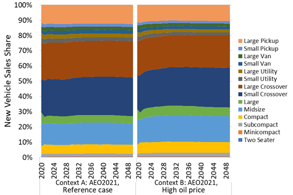
Fig. 4.3 Exogenous projections of size class from ‘context_new_vehicle_market.csv’
All vehicle attributes which are not explicitly projected exogenously and not modeled internally are held constant from the base year fleet. For example, while size class projections are provided for overall new sales in each year, the projections are not defined at the individual producer level. Therefore, MY2019 base year relative shares of size classes for each producer are assumed to hold constant in the future. As shown in the left bar chart of Fig. 4.4, in MY2019 OEM A was more heavily focused on the Large Pickup, Small Utility, and Small Crossover classes, while OEM B was more heavily focused on the Large Utility and Midsize car classes. These relative differences between producers are maintained in the model during the process of applying the size class projections for new sales overall to the individual vehicle projections, and their associated producers, in the base year. The result is shown on the right of Figure Fig. 4.4. The combined sales of OEM A and OEM B will match the overall new sales size class shares from Fig. 4.3, while retaining the relative tendency for OEM A and OEM B to produce different size class mixes.
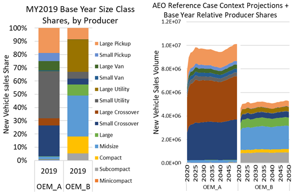
Fig. 4.4 Context size class projections applied to MY2019 base year vehicles
4.2. Policy Module
OMEGA’s primary function is to help evaluate and compare policy alternatives which may vary in terms of regulatory program structure and stringency. Because we cannot anticipate all possible policy elements in advance, the code within the Policy Module is generic, to the greatest extent possible. This leaves most of the policy definition to be defined by the user as inputs to the model. Where regulatory program elements cannot be easily provided as inputs, for example the equations used to calculate GHG target values, the code has been organized into user-definable submodules. Much like the definitions recorded in the Code of Federal Regulations (CFR), the combination of inputs and user-definable submodules must unambiguously describe the methodologies for determining vehicle-level emissions targets and certification values, as well as the accounting rules for determining how individual vehicles contribute to a manufacturer’s overall compliance determination.
Fig. 4.5 shows the flow of inputs and outputs for the Policy Module. As shown in this simple representation, the vehicle GHG targets and achieved certification values are output from the module, as a function of the attributes of candidate vehicles presented by the Producer Module.
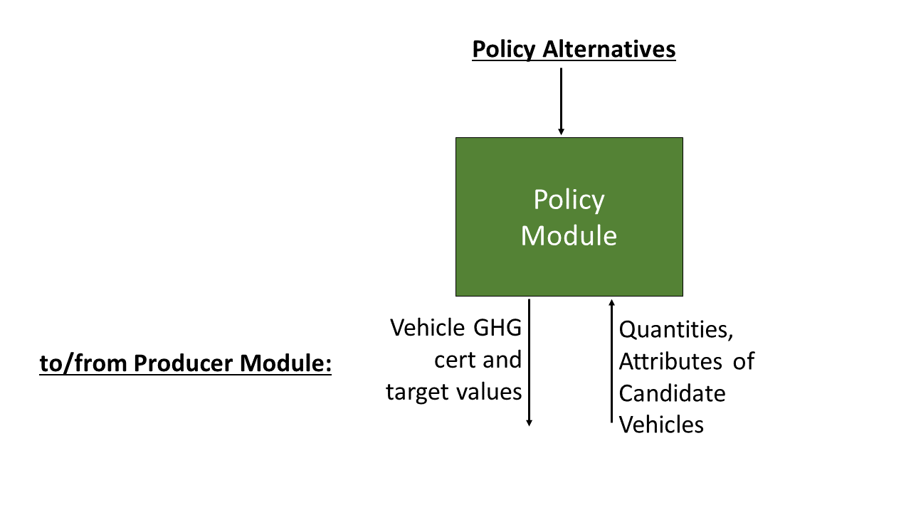
Fig. 4.5 Overview of the Policy Module
Throughout OMEGA, policy alternatives refer only to the regulatory options that are being evaluated in a particular model run. There will also be relevant inputs and assumptions which are technically policies but are assumed to be fixed (i.e. exogenous) for a given comparison of alternatives. Such assumptions are defined by the user in the analysis context, and may reflect a combination of local, state, and federal programs that influence the transportation sector through regulatory and market-based mechanisms. For example, these exogenous context policies might include some combination of state-level mandates for zero-emissions vehicles, local restrictions or fees on ICE vehicle use, state or Federal vehicle purchase incentives, fuel taxes, or a carbon tax. A comparison of policy alternatives requires that the user specify a no-action policy (aka context policy) and one or more action alternatives.
Policy alternatives that can be defined within OMEGA fall into two categories: those that involve fleet average emissions standards with compliance based on the accounting of credits, and those that specify a required share of a specific technology. OMEGA can model either policy type as an independent alternative, or model both types together; for example, in the case of a policy which requires a minimum share of a technology while still satisfying fleet averaging requirements.
Policy alternatives involving fleet average emissions standards: In this type of policy, the key principle is that the compliance determination for a manufacturer is the result of the combined performance of all vehicles, and does not require that every vehicle achieves compliance individually. Fleet averaging in the Policy Module is based on CO2 credits as the fungible accounting currency. Each vehicle has an emissions target and an achieved certification emissions value. The difference between the target and certification emissions in absolute terms (Mg CO2) is referred to as a credit, and might be a positive or negative value that can be transferred across years, depending on the credit accounting rules defined in the policy alternative. The user-specified policy inputs can be used to define restrictions on credit averaging and banking, including limits on credit lifetime or the ability to carry a negative balance into the future. The analogy of a financial bank is useful here, and OMEGA has adopted data structures and names that mirror the familiar bank account balance and transaction logs.
OMEGA is designed so that within an analysis year, under an unrestricted fleet averaging policy, credits from all the producer’s vehicles are counted without limitations towards the producer’s credit balance. Vehicles with positive credits may contribute to offset other vehicles with negative credits. The OMEGA model calculates overall credits earned in an analysis year as the difference between the aggregate certification emissions minus the aggregate target emissions. An alternative approach of calculating overall credits as the sum of individual vehicle credits is unnecessary and in some cases may not be possible. To give one example, if a policy applies any constraints on the averaging or transfer of credits, it would not be possible to determine compliance status simply by counting each vehicle’s credit contribution fully towards the overall credits.
The transfer of credits between producers can be simulated in OMEGA by representing multiple regulated entities as a hypothetical ‘consolidated’ producer, under an assumption that there is no cost or limitation to the transfer of compliance credits among entities. OMEGA is not currently designed to explicitly model any strategic considerations involved with the transfer of credits between producers.
Emissions standards are defined in OMEGA using a range of policy elements, including:
- rules for the accounting of upstream emissions
- definition of compliance incentives, like multipliers
- definition of regulatory classes
- definition of attribute-based target function
- definition of the vehicles’ assumed lifetime miles
Demo example: Input files for no-action and action policy definitions
| Policy element | No-action policy [Action policy] input files | Description |
|---|---|---|
| Drive cycles | drive_cycles-alt0[alt1].csv; drive_cycle_weights-alt0[alt1].csv | Drive cycle ID’s and weights for calculating weighted average emissions from certification tests. |
| Fuels | policy_fuels-alt0[alt1].csv | Direct and indirect CO2 values used in certification calculations for each fuel. |
| GHG credit rules | ghg_credit_params-alt0[alt1].csv | Credit carry-forward and carry-back rules. |
| GHG targets | ghg_standards-alt0[alt1].csv | Formula definitions for calculating g CO2/mi targets from vehicle attributes and regulatory classes. Also includes lifetime VMT assumptions. |
| Offcycle credits | offcycle_credits-alt0[alt1].csv | Offcycle credit values for specific technologies. |
| Upstream emissions accounting | policy_fuel_upstream_methods-alt0[alt1].csv | Selection of which methods to use for the calculation of indirect emissions certification values. |
| Advanced technology multipliers | production_multipliers-alt0[alt1].csv | Values for multipliers used in credit calculations to incentivize the introduction of specific technologies. |
| Reg classes | regulatory_classes-alt0[alt1].csv | Regulatory class ID’s and descriptions. |
| Technology mandates | required_sales_share-alt0[alt1].csv | Minimum required production shares as required by the policy. |
Policy alternatives requiring specific technologies: This type of policy requires all, or a portion, of a producer’s vehicles to have particular technologies. OMEGA treats these policy requirements as constraints on the producer’s design options. This type of policy alternative input can be defined either separately, or together with a fleet averaging emissions standard; for example, a minimum Zero Emission Vehicle (ZEV) share requirement could be combined with an emissions standard where the certification emissions associated with ZEVs are counted towards the producer’s achieved compliance value.
Policy representation in the analysis context: Some policies are not modeled in OMEGA as policy alternatives, either because the policy is not aimed directly at the producer as a regulated entity, or because the particular OMEGA analysis is not attempting to evaluate the impact of that policy relative to other alternatives. However, even when a policy is not reflected in any of the analyzed policy alternatives, it may still be appropriate to represent that policy in the Analysis Context inputs. This is especially true when that external policy (or policies) might significantly influence the producer or consumer decisions. Some examples include:
- Fuel tax policy
- State and local ZEV policies
- Vehicle purchase incentives
- Investment in refueling and charging infrastructure
- Accelerated vehicle retirement incentives
4.3. Producer Module
4.3.1. Producer Module Overview
The modeling of producer decisions is central to the optimization problem that OMEGA has been developed to solve. In short, the objective is to minimize the producers’ generalized costs subject to the constraints of regulatory compliance and consumer demand. The ‘producer’ is defined in OMEGA as a regulated entity that is subject to the policy alternatives being modeled, and responsible for making decisions about the attributes and pricing of new vehicles offered to consumers. A user might choose to model producers as an individual manufacturer of light duty vehicles, as a division of a single manufacturer, or as a collection of manufacturers. This choice will depend on the goals of the particular analysis, and what assumptions the user is making about the transfer of compliance credits within and between manufacturers.
Fig. 4.6 shows the flow of inputs and outputs for the Producer Module. Analysis context inputs are not influenced by the modeling within the Consumer, Producer, and Policy Modules, and are therefore considered as exogenous to OMEGA.
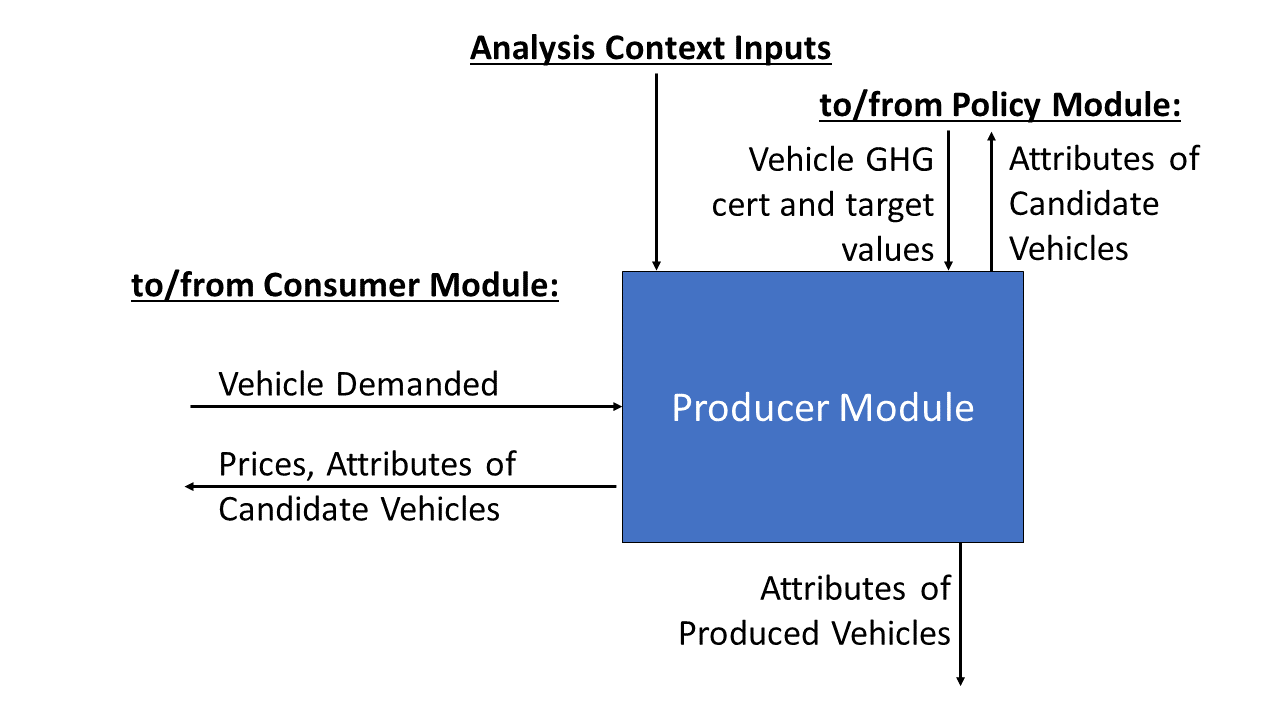
Fig. 4.6 Overview of the Producer Module
Inputs to the Producer Module: Policy Alternative inputs are used to calculate a compliance target for the producer (in Mg CO2) for a given analysis year using the provided attribute-based vehicle GHG targets, vehicle regulatory class definitions, and assumed lifetime VMT for compliance. Other policy inputs may define, for example, the credit lifetime for carry-forward and carry-back, or a floor on the minimum share of ZEV vehicles produced.
Analysis context inputs and assumptions that the Producer Module uses define all factors, apart from the policies under evaluation, that influence the modeled producer decisions. Key factors include the vehicle costs and emissions for the technologies and vehicle attributes considered, and the producer constraints on pricing strategy and cross-subsidization.
During the iteration process, shares of new vehicles demanded are generated by the Consumer Module as inputs to the Producer Module. These shares are at the market class-level, and based on the prices and attributes of the candidate vehicles offered by the producer in that iteration. See Section 4.5 for a description of the iteration and convergence algorithms.
Outputs of the Producer Module: During the iteration process, the outputs of the Producer Module describe the candidate vehicles – prices, quantities, and key attributes – which forms the basis for determining compliance status (by iterating with the Policy Module) and demanded sales shares (by iterating with the Consumer Module.) Once model convergence is achieved, the Producer Module outputs the details of the produced vehicles.
4.3.2. Producer Compliance Strategy
The Producer Module simulates decisions about vehicle design, pricing, and production quantities that minimize compliance costs while satisfying other considerations imposed by the policy, consumers, and production constraints. With a fleet averaging policy that allows credit banking and trading, the producer is making these product decisions within an overall strategy of managing compliance credits from year-to-year.
Vehicle design strategy
While the producer’s modeled objective function is cost minimization, the term ‘cost’ is used generically here, as it is not necessarily the case that the lowest production cost option is the best option for the producer. Consumer willingness to pay for a particular vehicle attribute can result in another choice if the producer expects that the additional production costs can be more than offset by a higher price. Here, the term producer generalized costs is defined as the net of vehicle production costs and the producer’s view of consumer’s willingness to pay for that vehicle.
The Producer Module will first attempt to select the available vehicle design options (i.e. tech package applications) and sales mix that minimizes generalized costs while meeting the strategic compliance target (Mg CO2e.) This is the starting point of an iterative process, since in many cases the demand estimated by the Consumer Module will not match this first set of vehicle attributes, prices, and quantities within the desired convergence tolerance.
Vehicle pricing and sales mix strategy
In addition to influencing key vehicle attributes by the design decisions, the producer also has some flexibility in how vehicle prices are set. Using cross-subsidization strategies to spur greater sales of some vehicles at the expense of others, producers can incentivize market class sales mix changes in order to reduce generalized costs. This assumption that producers will attempt to minimize their generalized costs is consistent with a producer goal of profit maximization.
In reality, there are limits to the ability of producers to adjust vehicle prices. The user can define upper and lower limits to how much price cross-subsidization can be applied. Also, the model automatically only searches for solutions that maintain the overall average vehicle price, thus forcing any cross-subsidization strategies to be revenue neutral.
Credit management strategy
With a policy that allows credit banking, the efficient management of compliance credits from year-to-year involves a degree of look-ahead, both in terms of expected changes in regulatory stringency and other policies, and expected changes in generalized costs over time. At this time, OMEGA assumes that producers aim to meet the GHG target in each year, with any banked credits used only to make up differences between the certification and target values. The producer logic associated with the process box labeled “Determine Strategic Target Offset” in the process flow diagram (Fig. 4.2) therefore simply applies the offset, if any, to the policy GHG target. In a future revision, we plan to consider incorporating producer decisions that are intentionally under- or over-target based on the assumption that producers make strategic decisions looking beyond the immediate present to minimize generalized costs over a longer time horizon.
4.3.3. Vehicle Definitions
The vehicle is the fundamental unit of analysis within the Producer Module, and the decisions made by producers determine the vehicle attributes and sales in the modeled results. The vehicle resolution is determined by the user (see Section 4.1.1) consistent with the resolution defined in the base year vehicles input file. Depending on the focus of a particular run, vehicles might be defined at a market class level using an aggregate representation over multiple producers, or at the nameplate or even subconfiguration level.
Along with a definition of resolution, the base year vehicles inputs also define the key exogenous attributes that are necessary for 1) generating future projections, 2) assigning the policy emissions targets, 3) estimating consumer demanded quantities, 4) determining appropriate emissions rates and costs from the applied technology packages.
Demo example: Vehicle definitions in base year fleet
| Field Name | Attribute Required For: | Example 1 | Example 2 | Example 3 | Example 4 |
|---|---|---|---|---|---|
| vehicle_name | tracking of producer decisions in modeled results | ICE Large car | ICE Large Crossover truck | ICE-HEV Large Pickup truck 4WD | ICE Large Van truck minivan 4WD |
| manufacturer_id | grouping for producer modeling | OEM_B | OEM_A | OEM_A | OEM_A |
| model_year | determination of analysis start year | 2019 | 2019 | 2019 | 2019 |
| reg_class_id | reference (assigned by policy in analysis timeframe) | car | truck | truck | truck |
| epa_size_class | reference | Large Cars | Standard SUV 2WD | Standard Pick-up Trucks 4WD | Special Purpose Vehicle, minivan 4WD |
| context_size_class | sales mix projections | Large | Large Crossover | Large Pickup | Large Van |
| electrification_class | reference (modeled element in analysis timeframe) | N | N | HEV | N |
| cost_curve_class | cost and emissions rates for tech packages | ice_MPW_LRL | ice_MPW_HRL | ice_Truck | ice_MPW_HRL |
| in_use_fuel_id | reference (modeled element in analysis timeframe) | {‘pump gasoline’:1.0} | {‘pump gasoline’:1.0} | {‘pump gasoline’:1.0} | {‘pump gasoline’:1.0} |
| cert_fuel_id | reference (modeled element in analysis timeframe) | {‘gasoline’:1.0} | {‘gasoline’:1.0} | {‘gasoline’:1.0} | {‘gasoline’:1.0} |
| sales | sales mix projections | 536531 | 496834 | 78297 | 13795 |
| cert_direct_oncycle_co2e_grams_per_mile | reference (modeled element in analysis timeframe) | 345.3 | 418.6 | 405.8 | 403.0 |
| cert_direct_oncycle_kwh_per_mile | reference (modeled element in analysis timeframe) | 0 | 0 | 0 | 0 |
| footprint_ft2 | policy targets (‘Alternative 0’ only) | 50.5 | 54.7 | 68.5 | 56.0 |
| eng_rated_hp | reference (modeled element in analysis timeframe) | 268 | 318 | 364 | 296 |
| tot_road_load_hp | reference (modeled element in analysis timeframe) | 12.5 | 16.1 | 19.3 | 17.3 |
| etw_lbs | reference (modeled element in analysis timeframe) | 4035 | 5095 | 5518 | 5000 |
| length_in | reference | 195.3 | 201.6 | 231.6 | 200.6 |
| width_in | reference | 73.8 | 78.0 | 80.6 | 78.1 |
| height_in | reference | 58.2 | 71.1 | 77.0 | 70.4 |
| ground_clearance_in | reference | 5.2 | 8.3 | 6.5 | |
| wheelbase_in | reference | 114.0 | 118.4 | 143.1 | 119.3 |
| interior_volume_cuft | reference | 148.3 | |||
| msrp_dollars | reference (modeled element in analysis timeframe) | 42554 | 46592 | 40740 | 39962 |
| passenger_capacity | policy targets (‘Alternative 1’ only) | 5.0 | 6.6 | 5.5 | 7.0 |
| payload_capacity_lbs | reference | 1030 | 1438 | 1748 | |
| towing_capacity_lbs | reference | 1000 | 5598 | 10509 | 3500 |
| unibody_structure | reference | 1 | 1 | 0 | 1 |
4.3.4. Vehicle Simulation and Cost Inputs
One of the most important sets of inputs to the Producer Module is the simulated vehicles file. It contains the vehicle parameters used by OMEGA to generate all possible vehicle technology (and cost) options available to the producers – these production options represent distinct points in what might be considered a point ‘cloud’. The use of these vehicle clouds by OMEGA is described in Section 4.3.5.
The simulated vehicle file contains the various vehicles of different core attributes (such as vehicle size, weight, powertrain, etc), the CO2-reducing technologies that are applied to each, and their predicted energy consumption, CO2 performance, and cost. While not required by all users, EPA uses its own simulation tool (ALPHA) to predict the energy consumption and CO2 emissions for each vehicle and technology combination. For the demo, these vehicle and technology options (and associated CO2 performance) are consolidated into the ‘simulated_vehicles.csv’ file. The simulated vehicles file contains the following fields for use in the Producer Module:
- the associated cost curve class (defined by powertrain family and described below)
- vehicle properties such as curb weight, type of base powertrain (ICE/HEV/PHEV/BEV, etc)
- other included technologies (e.g., A/C credits, high efficiency alternator, etc)
- test cycle performance (energy consumption (for plug-in vehicles) and/or CO2 emissions)
- vehicle attributes, such as included technologies, costs
Significance of the cost curve class: Each cost curve class includes multiple vehicles and represents the design space for all vehicle options in each class. In the demo, multiple vehicles are grouped within a single cost curve class to reduce the number of simulations required to represent the design space. OMEGA producer decisions are made based on discrete vehicle options within each vehicle cost curve class. For possible future consideration, EPA recommends the generation of RSEs (response surface equations) to derive particular cost clouds unique to each vehicle. This would allow for more unique cost and vehicle clouds without excessive simulation calculation burden.
4.3.5. Vehicle Cost Clouds, Cost Curves, and Aggregation
The technology packages and their application to candidate vehicles are described in the model inputs as a discrete set of options that were generated using tools and approaches external to OMEGA (e.g. vehicle simulation, benchmarking, cost teardowns, etc.) Because the product design problem being solved is multi-dimensional (i.e. an intersection of technology package applications and market share decisions for multiple vehicles), the choice set must be built up from various combinations of vehicle-level decisions that cannot be readily predicted in advance.
The Producer Module uses an approach of aggregating the discrete, vehicle-level decisions at several levels, while retaining the vehicle-specific information that can be accessed later in other stages of the modeling and presented in the results. These processes of vehicle aggregation (also referred to as composition or the creation of “composite vehicles”) and decomposition are critical for the solution search process. First, aggregation allows the model to efficiently search for a solution without a complete enumeration of all possible choice combinations. Second, decomposition allows the model to draw upon the key vehicle attribute details that have been retained and are required for calculating the compliance emissions values and estimating the consumer response.
Vehicle-level technology application options
In oder to minimize cost, a producer would need to select the minimum cost package available at a given compliance emissions rate (i.e. g CO2/mi.) This subset of cost-minimizing vehicle technology packages is referred to as the cost curve, while the broader set of points is the cost cloud. Note that ‘cost’ here is referring to the producer generalized cost, as explained in Section 4.3.2.
Demo example: Vehicle cost clouds
An example cost cloud for a single vehicle in MY2025 (vehicle #62, a 4WD minivan) for the no-action policy in Context A is shown in Fig. 4.7. The costs for the blue points are production costs. The orange point costs are producer generalized costs, and include 5 years of fuel costs at 15,000 miles per year that the producer assumes are valued by consumers at the time of purchase (as defined in the analysis context input file ‘producer_generalized_costs.csv’.) Note that the producer generalized costs are higher than the production costs, and also form a cloud with a different shape than the blue production cost cloud. Essentially, the orange cloud is shifted up and rotated counterclockwise relative to the blue cloud because the technology packages with higher emissions rates also have relatively higher fuel costs that are assumed to factor into consumer purchases.
Fig. 4.7 also contains the resultant cost curve (black line) that represents the cost-minimizing frontier of the cost cloud. The Producer Module automatically generates this piece-wise linear approximation of the frontier using points in the cloud.
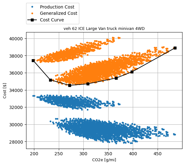
Fig. 4.7 Example vehicle cloud
Compliance options based on design decisions across multiple vehicles
Because a producer can offer a range of different vehicles, each with distinct costs associated with applying technology packages, it is not likely that the lowest cost compliance solution will be a uniform application of technology to all vehicles. Nor will selecting the lowest cost option for each vehicle likely result in producer compliance, except in cases where a policy is non-binding. In order to consider design options for multiple vehicles simultaneously, the Producer Module aggregates individual vehicles into composites, with one composite vehicle for each market class and reg class combination. It is important that the resultant cost curves (producer generalized cost vs. g CO2/mi emissions rates) are not aggregated further since 1) aggregating emissions rates across market classes would no longer be valid after iteration when the Consumer Module changes the relative shares of market classes, and 2) aggregating emissions rates across regulatory classes would, under some policy definitions, make it impossible to calculate the Mg CO2 compliance credits (e.g. in policy cases where there are limits to the transfer of credits between regulatory classes.)
Demo example: Vehicle aggregation into market class - reg class cost curves
Fig. 4.8 shows the black cost curve of veh #62 as presented in Fig. 4.7, along with the other vehicles that are in the same combination of market class (ICE non-hauling) and reg class (‘a’.) Note that the simulated_vehicles.csv file for this demo example does not contain distinct costs and emissions rates for every vehicle. As a result, even though there are 12 vehicles are represented here, they overlay into only three distinct cost curves. If a user provided simulated_vehicles.csv inputs defined with greater resolution, every vehicle could be associated with its own distinct cost curve.
The bold orange line in Fig. 4.8 is the MY2025 cost minimizing frontier for a composite vehicle made by aggregating the individual vehicle cost curves in the same market class and reg class combination. The relative shares of vehicles within a market class and reg class remain fixed in the Producer-Consumer iteration process. Therefore the composite vehicle cost curve does not change as a result of the consumer response. This curve, along with the composite vehicle cost curves from the other market class and reg class combinations, is used to generate the producer compliance options.
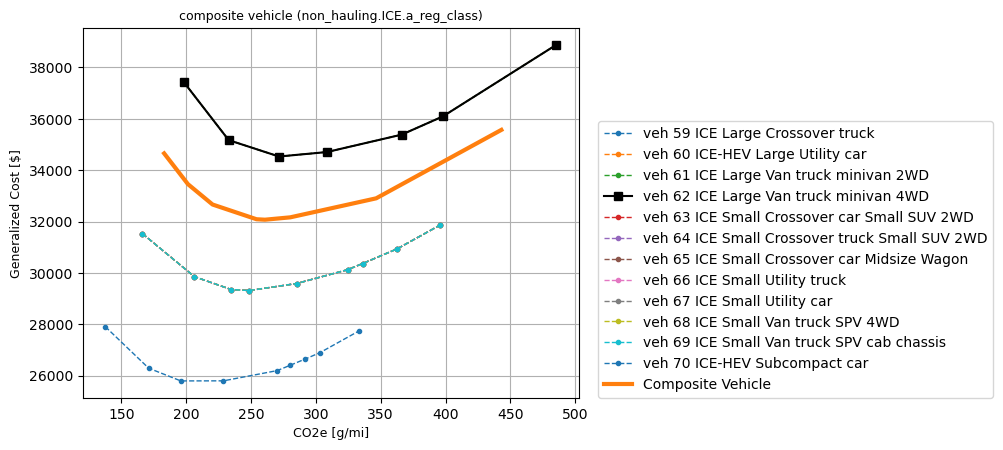
Fig. 4.8 Example aggregation of vehicles into a composite vehicle
Once composite vehicle cost curves are generated for each market class and reg class combination, the Producer Module creates compliance options from a combination of design choices for the relative shares of composite vehicles and the emissions rate of each composite vehicle. The resulting compliance options are defined in terms of cost vs. Mg CO2 credits rather than g CO2/mi. See Section 4.5 (iteration and convergence) for more discussion of how the model converges on a solution by searching among these compliance options, and generating interpolated compliance options that are successively more refined with each iteration.
Extracting key vehicle attributes from the composite vehicles through decomposition
Once a compliance option is selected through the iteration and convergence process, a user will likely want to know how specific vehicle design decisions contributed to that solution.
Demo example: Decomposition of composite vehicle
Because the composite vehicle is made up of individual vehicles of fixed sales shares (at least relative to the other vehicles in the same market class, reg class combination), there is one-and-only-one solution for individual vehicle costs and emissions rates that will result in the selected option for the composite vehicle’s cost and emissions rate. Fig. 4.9 shows the same orange composite vehicle curve from Fig. 4.8, along with star symbols to indicate the selected option for the composite vehicle and associated points for the individual vehicles.
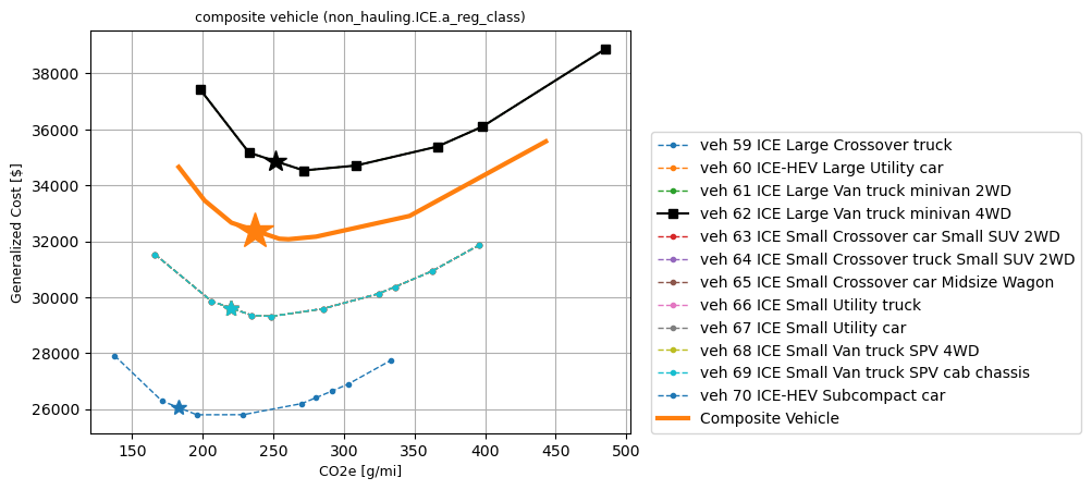
Fig. 4.9 Example decomposition of composite vehicle back to individual vehicles
4.4. Consumer Module
The Consumer Module is a significant addition to OMEGA. With the ongoing evolutions in the light-duty vehicle market, including major growth in technologies and services, the need for an endogenous consumer response is clear. The Consumer Module is structured to project how consumers of light-duty vehicles would respond to policy-driven changes in new vehicle prices, fuel operating costs, trip fees for ride hailing services, and other consumer-facing elements. The module is set up to allow the inputs to affect total new vehicle sales (both in number and proportion of sales attributes to different market classes), total vehicle stock (including how the used vehicle market responds), and total vehicle use (the VMT of the stock of vehicles).
An important consideration with the addition of the Consumer Module is ensuring consistency between the set of vehicles and their attributes that the Producer Module supplies and the set of vehicles and their attributes that the Consumer Module demands. In order to estimate the set of new vehicles that provide this equilibrium, the Consumer and Producer modules iterate until convergence is achieved - where the set of vehicles, including their prices and attributes, that satisfy producers is the same set of vehicles that satisfy consumers.
4.4.1. Consumer Module Overview
As explained in the Overview chapter, and shown in Fig. 1.1, OMEGA is structured in a modular format. This means that each primary module — the Policy Module, Producer Module, Consumer Module and Effects Module — can be changed without requiring code changes in other modules. This ensures users can update model assumptions and methods while preserving the consistency and functionality of OMEGA.
An overview of the Consumer Module can be seen in Fig. 4.10. This overview shows the connections between the Consumer Module, the analysis context, and other OMEGA modules. The Consumer Module receives inputs from the analysis context and the Producer Module, and computes outputs used in iteration with the Producer Module and for use in the Effects Module.
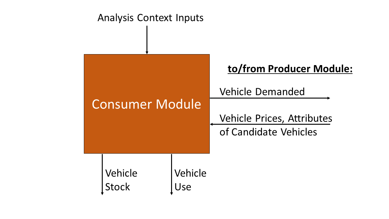
Fig. 4.10 Overview of the Consumer Module
The Consumer Module’s purpose is to estimate how light duty vehicle ownership and use respond to key vehicle characteristics within a given analysis context. There are five main user-definable elements estimated within the Consumer Module, as seen in Fig. 4.11. These estimates are: market class definitions, new sales volumes, new vehicle sales shares by market class (where market classes depend on the requirements of the specific consumer decision approach used in the analysis), used vehicle market responses (including reregistration), and new and used vehicle use measured using vehicle miles traveled (VMT). Further explanations of each of these elements are described in the following sections.
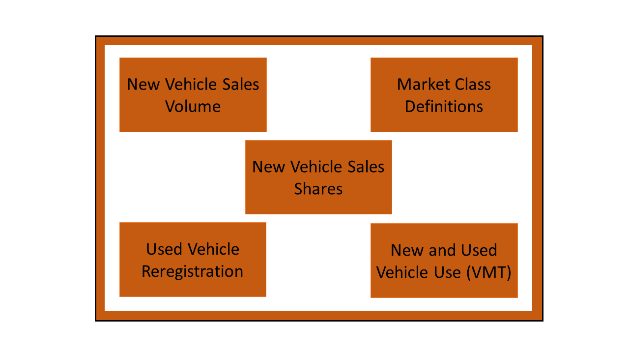
Fig. 4.11 Inside the Consumer Module
Each of these five elements represents a user-definable submodule within the Consumer Module code. The code within each submodule may be updated by a user, or the submodule may be replaced with an alternative submodule. When a modifies a submodule, they must ensure that the submodule retains consistency with the other submodules within the Consumer Module, as well as with the rest of OMEGA. For example, if the market class submodule is changed from the demo analysis version, the sales share submodule must be updated as well since sales shares are determined by market class.
Demo example: Consumer Module user-definable submodules
The user-definable submodules in the demo analysis version of the Consumer Module are listed in the table below.
| Element | Submodule |
|---|---|
| Market class definitions | market_classes.py |
| New vehicle sales volume | sales_volume.py |
| New vehicle sales shares | sales_share.py |
| Used vehicle reregistration | reregistration_fixed_by_age.py |
| New and used vehicle use | annual_vmt_fixed_by_age.py |
The Consumer Module works in two phases: first, an iterative new vehicle phase, followed by a non-iterative stock and use phase. During the first phase, the Consumer Module and Producer Module iterate to achieve convergence on the estimates of new vehicles produced and demanded that meet the standards set in the Policy Module. The Producer Module sends a set of candidate vehicles, including their prices and attributes, to the Consumer Module to consider. The Consumer Module uses that set of candidate vehicles to estimate total new vehicles demanded and the shares of those new vehicles in the specified market classes, which are passed back to the Producer Module. If the estimates do not converge within a tolerance, a new set of candidate vehicles is sent to the Consumer Module for consideration. See Section 4.5 for more information on the Consumer-Producer iteration process. Once convergence between the Producer and Consumer modules is achieved, the set of candidate vehicles are no longer considered candidates for consideration, but are the estimated new vehicle fleet, and the Consumer Module enters the second phase. In this phase, total vehicle stock (new and used vehicles and their attributes) and use (VMT) are estimated.
Inputs to the Consumer Module In general, the Consumer Module uses exogenous inputs from the analysis context, and endogenous inputs from the Producer Module. The exogenous inputs may include data such as fuel prices, existing vehicle stock, and specific modeling parameters, for example, the parameters used in estimations of vehicle ownership and use decisions. The analysis context must also contain the inputs required to define projections of vehicle ownership and use in the absence of any policy alternatives being analyzed. These projections might be provided directly as inputs to the Consumer Module, such as projections of vehicle ownership from the Annual Energy Outlook (AEO), or generated within the Consumer Module based on exogenous inputs, including future demographic or macroeconomic trends. Endogenous inputs are factors determined within the model and passed to the Consumer Module from the Producer Module. They may include vehicle prices and other relevant vehicle attributes, such as fuel consumption rate. Because the Consumer Module’s internal representation of consumer decisions can be defined by the user, the specific exogenous and endogenous inputs required will depend on the models, methods, and assumptions specified by the user. The vehicle attributes needed as inputs to the Consumer Module are determined by the methods used to estimate new vehicle sales, the market shares of vehicles demanded, used vehicle reregistration, and new and used vehicle use. For example, vehicle attributes used to define market classes must be included as inputs from the Producer Module. As an additional example, if the user defines vehicle sales responses to differ based on consumer income, the user must ensure that income is included in the analysis context inputs.
Outputs of the Consumer Module The Consumer Module produces two categories of outputs: sales estimates during the iterative Phase 1, and stock and use estimates during the non-iterative Phase 2. During the iterative phase, outputs of the Consumer Module, including new vehicle sales and responsive market shares (explained in the following section), are fed back to the Producer Module for iteration and convergence. See Section 4.4.3 for more information on what happens during Phase 1, and Section 4.5 for more detailed information on how OMEGA estimates iteration and convergence between the Producer and Consumer modules. Once that convergence is achieved, the Consumer Module estimates the outputs of the stock of vehicles, including both new and reregistered used vehicles, and VMT, which are used by the Effects Module.
4.4.2. Market Class Definitions
During the iterative first phase, the Consumer Module considers vehicle prices and attributes at an aggregate level by grouping vehicles into market classes. These market classes are the fundamental unit of analysis for which the Consumer Module estimates new vehicle sales and shares. The choice of market classes is tied to the specification used to estimate the shares of new vehicles sold, and is dependent on the attributes available in the input data files. For example, vehicles might be identified by attributes such as fuel type (electric, gas, diesel, etc.), expected use (primarily for goods or passenger transport), or size.
Users can define market classes in the market class definitions submodule (as shown in Fig. 4.11.) In doing so, the user must ensure that all other inputs and user-definable submodules (for example, with respect to stock and use estimation) within the Consumer Module are defined consistently. For example, if the sales share submodule is defined as estimating shares of vehicles in a set of fuel type categories, those fuel type categories must be defined within the market class submodule.
The designation of market classes can be used to reflect market heterogeneity in purchasing behavior or vehicle use based on specific vehicle attributes. Accordingly, market classes are defined using vehicle attributes and inputs from the analysis context (i.e. the base year vehicle inputs.) In addition, the user can categorize market classes as ‘responsive,’ where the shares of total vehicles attributed to those market classes change due to endogenously modeled elements that change in response to policy (like relative costs), or ‘nonresponsive,’ where the shares of total vehicles attributed to those market classes do not change with the policy being analyzed.
Before the Consumer Module can estimate new vehicle sales or market shares responses, all vehicles must be categorized into their market classes. This categorization is defined as a series of nested market category levels. The user can define any number of market classes, or levels, as well as the hierarchy of the levels. In defining the hierarchy, it is important to note that OMEGA assumes that the sales share estimates within a parent category are independent of sales share estimates outside the parent category. This means that changing the available market classes outside the parent category will not change the sales share estimates within the parent category.
Demo example: Market class structure
Fig. 4.12 below illustrates an example of a nested market class hierarchy using the demo analysis market classes as an example. Hauling/non-hauling market classes are the highest, parent, level. Vehicles are separated into the appropriate hauling and non-hauling class using their attributes. Nested within the hauling and non-hauling categories, there are BEV/ICE market classes. The candidate vehicle inputs from the Producer Module, for example, vehicle prices, fuel cost and VMT, are used to determine the share of vehicles in the BEV/ICE market classes, as described in the examples below. During the iterative first phase, if the share of BEVs that consumers will accept given the candidate vehicle attributes does not converge within a tolerance with the share that the Producer Module estimates, the iterative process continues. The demanded BEV share is passed back to the Producer Module, which will return a new set of candidate vehicles and their attributes, including prices. Given the updated candidate vehicle inputs, the Consumer Module will redistribute vehicles into the BEV and ICE classes, with the BEV/ICE share estimates in the hauling category being independent from those in the non-hauling category. This possible redistribution between market class categories is represented by the dashed lines between each set of BEV/ICE classes. Note that the dashed lines travel within the hauling class and within the non-hauling class, but do not travel across them.
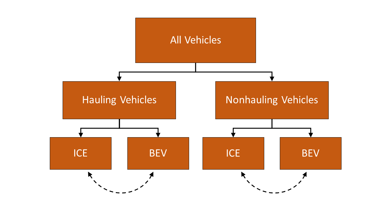
Fig. 4.12 Illustration of the Market Class Structure in the Demo Analysis
Within a given analysis context, the shares of vehicles allocated to nonresponsive market class categories do not shift between those nonresponsive market categories, even under different policy alternatives or during iteration with the Producer Module. Shares of vehicles allocated to responsive market class categories may shift between the responsive market categories.
Demo example: Nonresponsive and responsive market classes
Within the demo analysis, vehicles are separated into four market classes depending on whether they are categorized as hauling (primarily meant for transporting goods or towing, as a body-on-frame vehicle would be expected to do) or non-hauling (primarily meant for passenger transportation, as a unibody vehicle might do), and their fuel type (battery electric vehicle (BEV) or internal combustion engine vehicles (ICE)). The hauling/non-hauling market classes are defined as nonresponsive market class categories. The share of vehicles defined as hauling or non-hauling, regardless of the fuel type, depends on analysis context inputs, and is unaffected by model results. The BEV/ICE market classes are defined as responsive market class categories, the share of vehicles in that market class is estimated within the Consumer Module and is responsive to vehicle cost and fuel consumption rate of the set of candidate vehicles input from the Producer Module.
4.4.3. Phase 1: Producer-Consumer Iteration
During the iterative first phase of the Consumer Module, the Producer Module and Consumer Module iterate to estimate total new vehicle sales, market shares, and prices at the market class level, based on the candidate vehicle options being offered by the producer. The iteration process is described more fully in the Iteration and Convergence Algorithms section. It begins with the Producer Module providing a set of candidate vehicles that meet the policy targets as defined within the Policy Module while minimizing the producer’s generalized costs. At this initial step, overall volumes are taken directly from the analysis context projections, along with sales shares projection of nonresponsive market class categories. If the sales and market shares result estimated within the Consumer Module is not within a given threshold of the estimates from the Producer Module, iteration between the modules occurs. The process entails the Producer Module offering successive sets of candidate vehicles and their attributes, including prices, which still achieve the policy targets until a there is set of candidate vehicles which results in agreement between the Producer Module and Consumer Module estimates of sales and market shares, or until an iteration limit is reached. On the Producer Module side, the process also includes determining the level of cross-subsidization between vehicle classes, which is covered more fully in the Iteration and Convergence Algorithms section. Within this iterative first phase of the Consumer Module, there are two main determinations being made: the total sales volume consumers will accept, and the share of vehicles they demand from each market class. Much of the method and assumptions used to estimate sales and shares impacts can be defined by the user in the New Vehicle Sales Volumes and New Vehicle Sales Shares submodule as seen in Fig. 4.11, including the method of estimating a change in sales volumes or responsive market shares, consumer responsiveness to price, and what is included in the price consumers take into account.
Sales volumes
The Consumer Module estimates the total new vehicles sold at the aggregated market class level with the user-definable submodule for new vehicle sales. The estimate for the change in new vehicle sales starts with an assumption of sales volumes in the Context Policy (the “no-action alternative”). These estimates can be an exogenous input from the analysis context, or estimated within the Consumer Module. Sales volumes under a defined policy (an “action alternative”) can be responsive to policy if the estimation is defined as relying, at least in part, on inputs from the Producer Module, or may be unresponsive to policy if the estimation is defined to rely solely on inputs from the analysis context. In defining how the Consumer Module estimates sales volumes, the user must ensure consistency between the inputs available from both the Producer Module and the analysis context, as well as with the other user-definable submodules within the Consumer Module. For example, if a user defines sales volumes as responsive to a specific vehicle attribute, that attribute must be included in the set of candidate vehicles and their attributes input from the Producer Module.
Demo example: New vehicle sales estimates
In the demo analysis, sales volumes under the no-action policy alternative, which is also the Context Policy, are an exogenous input from the analysis context. An elasticity of demand, defined by the user, is used in conjunction with the change in price between a no-action alternative and an action alternative to estimate the change in sales from the no-action alternative level. Demand elasticity is defined as the percent change in the quantity of a good demanded for a 1% change in the price of that good, where the good demanded in the Consumer Module is new light duty vehicles. They are almost always negative: as the price of a good increases (a positive denominator), the amount of that good purchased falls (a negative numerator). Larger (in absolute value) negative values are associated with more “elastic”, or larger, changes in demand for a given change in price. This value represents how responsive consumers are to a change in price. The general elasticity equation is:
Where:
- \(E_D\) is the elasticity of demand
- \(\Delta Q\) is the change in the quantity demanded
- \(Q\) is the quantity demanded before the price changes
- \(\Delta P\) is the change in the good’s price
- \(P\) is the good’s price before the change
In the demo analysis, the default elasticity of demand is set to -1. This means, for a 1% change in the consumer generalized price (described below), the vehicles demanded by consumers will fall by 1%. In order to estimate the change in sales expected as function of the estimated change in price, this equation is rearranged:
At an aggregate level, the average expected change in the price of new vehicles is multiplied by the defined demand elasticity to get the estimated change in vehicles demanded. This change is combined with projected new vehicle sales under the no-action alternative to get the total new vehicle sales under the action alternative outlined in the Policy Module.
If a user adopts the demo analysis method of estimating sales volumes using an elasticity of demand, they must ensure that net vehicle price, P, is defined. This net price is estimated under the no-action and the action alternatives, and the no-action alternative net price is subtracted from the action alternative net price to get an estimated change in net price, \(\Delta P\), that can be used with the user-specified elasticity. The net price should include factors the user assumes consumers consider in their purchase decision. Some factors that might be included are the share of total costs the producers pass onto the consumers, and the amount of future fuel costs consumers consider in their purchase decision.
Demo example: Net price
In the demo analysis, the net price value in the sales volume estimate includes assumptions about the share of the total cost that producers pass onto the consumer and the amount of fuel consumption considered in the purchase decision. With respect to the share of total cost that producers pass onto consumers, the demo analysis assumes “full cost pass-through.” This means that the full increase in cost that producers are subject to in achieving emission reduction targets is passed on to the consumers. However, due to cross-subsidization, those costs may be spread across multiple market classes.
The role of fuel consumption in the purchase decision is represented by the number of years of fuel consumption consumers consider when purchasing a new vehicle, and can range from 0 through the full lifetime of the vehicle. Fuel costs are estimated using vehicle fuel consumption rates from the Producer Module, projections of fuel prices from the analysis context, the user-specified VMT schedules, and the user-specified vehicle reregistration schedules. The resulting portion of fuel costs considered by consumers is added to the candidate vehicle prices from the Producer Module to produce a net vehicle price, which is then used in conjunction with the elasticity of demand to estimate the change in vehicle sales. The demo analysis assumes that consumers consider 5 years of fuel costs in the vehicle purchase decision.
Sales shares
The new vehicles sold are categorized into the user-definable market classes using estimates of sales shares. As mentioned above, those market classes can be nonresponsive or responsive to the policy being analyzed. Nonresponsive vehicle shares do not change with updated candidate vehicle sets or across policy alternatives. Though not responsive to endogenous inputs, the nonresponsive sales shares do not have to be constant. For example, they may be provided as a set of values for different points in time if the shares are expected to change exogenously over time. In addition, users can define sales shares to explicitly consider consumer heterogeneity by defining separate sales share estimates for different consumer groups. For example, sales share responses can differ between rural and urban consumers. If users identify heterogenous consumer groups with separate sales share responses, the analysis context must include the appropriate inputs. For example, the proportion of the vehicle buying population in urban and rural areas for each year being analyzed within the model.
For responsive market classes, users can define how market shares are responsive to attributes of candidate vehicle sets fed in from the Producer Module, for example vehicle price. In addition, the inputs used to estimate shares must be available within the set of candidate vehicles and their attributes, or as part of the analysis context.
If the user retains the demo analysis method of determining responsive BEV shares (using a logit curve as described above), the parameters representing the speed of acceptance, \(\alpha_{i}\), and price responsiveness, \(\gamma\), are factors the user can modify in the sales share submodule inputs (see sales share inputs)
In addition, the user must specify the price used in the logit equation. This price should include factors the user estimates are significant in determining relative market shares; cost factors can be monetary, such as capital and maintenance costs, or non-monetary, such as time. In addition, price estimation needs to be consistent with the speed of acceptance and price responsiveness parameters.
4.4.4. Phase 2: Vehicle Stock and Use
If convergence with respect to the sales and shares of new vehicles is achieved, the Consumer Module estimates total vehicle stock and use. To do so, it needs to keep internal consistency between- the number of vehicles demanded and the use of those vehicles. The method of determining total vehicle stock and vehicle use are in user-definable submodules represented by the used vehicle market response element and the new and used vehicle use element in Fig. 4.11. Vehicle stock is the total onroad registered fleet, including both new vehicles sales and the reregistered (used) vehicles. The data contained in the set of vehicle stock includes both vehicle count, as well as the attributes of the vehicles in the set, including model year and the vehicle features or attributes used to designate market classes. Vehicle use is the measure of how much each vehicle is driven in the analysis year, measured in vehicle miles traveled (VMT). VMT is determined at the vehicle level.
Vehicle stock
Fig. 4.13 below steps through the flow of how total vehicle stock is estimated in OMEGA. To estimate vehicle stock, the model starts with a base year stock of vehicles, which is an input from the analysis context. The base year is the last year actual observations, and is unmodified during the analysis. The analysis start year is the first year in which modeling is performed and immediately follows the base year. The stock of vehicles at the end of the analysis start year includes the new vehicles produced, plus the set of vehicles that were reregistered from the base year stock. For each subsequent modeled (analysis) year, the total stock is determined from the new vehicles produced in that year plus the reregistered vehicles from the prior year.
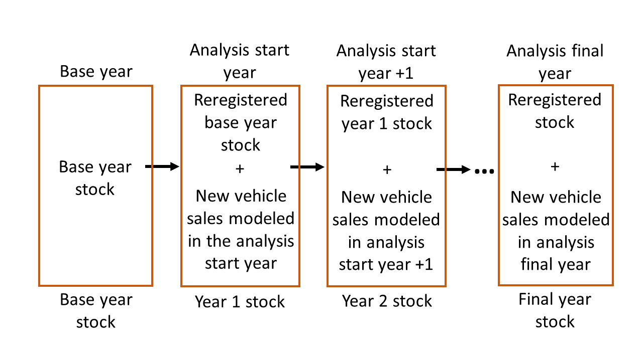
Fig. 4.13 Vehicle stock estimation flow diagram
The method of estimating the reregistered fleet is in a user-definable used vehicle reregistration submodule. This method can make use of a static schedule, for example, where a vehicle’s age is the only determinant of the proportion of vehicles remaining in the fleet over time, or depend on other vehicle attributes, like cumulative VMT. If users modify the reregistration submodule to follow a different prescribed static rate, or to allow interdependencies between the rate of reregistration and other vehicle attributes, they need to retain consistency between the reregistration submodule and other submodules, for example the submodules estimating new vehicle sales and total VMT.
Demo example: Vehicle stock estimates
In the demo analysis, the analysis start year stock of vehicles comes from the analysis context, and reregistration is estimated using fixed schedules based on vehicle age. For every calendar year, a specified proportion of vehicles in each model year is assumed to be reregistered for use in the following calendar year. In this fixed schedule, the proportion of vehicles of a given model year remaining in the registered stock (i.e. the survival rate) falls as the vehicles age. For example, in 2030, the proportion of the original MY 2025 vehicles remaining is larger than the proportion of MY 2015 vehicles remaining.
Vehicle use
Vehicle use is estimated as the vehicle miles traveled for each vehicle in the stock for the analysis year. This can be thought of as a measure of consumer demand for mobility. The method of estimating total VMT for the stock of vehicles is in a user-definable new and used vehicle use submodule. VMT can be estimated simply as a function of vehicle age, or may be a function of age, market class, analysis context inputs or more. Use could also include estimates of rebound driving. Rebound driving is estimated as the additional VMT consumers might drive as a function of reduced cost of driving.
Demo example: VMT estimates
In the demo analysis, total VMT demanded is an input from the analysis context and is constant across policy alternatives. Total VMT demanded is combined with the initial stock of vehicles and their attributes from the analysis context to determine the proportion of VMT attributed to cohorts of vehicles separated by age and market class. For each calendar year, the total VMT projected in the analysis context is allocated across the internally estimated stock of vehicles using this fixed relationship. This method allows VMT per vehicle to change with the total stock of vehicles, while assuming that consumer demand for mobility is not affected by the action alternatives under consideration. The demo analysis does not currently implement VMT rebound estimations.
4.5. Iteration and Convergence Algorithms
OMEGA finds a solution in each analysis year using iterative search algorithms. As shown in the process flow diagram in Fig. 4.2, the model uses two iterative loops; a Producer-Policy loop and a Producer-Consumer loop. For both loops, convergence criteria must be achieved within a specified tolerance for the simulation to proceed. This section describes those loops in more detail, with additional information from the demo example.
‘Producer-Policy’ Iteration: Compliance Search
The iteration process begins with a search for the vehicle design options and market class shares that minimize producer generalized costs and achieve the desired compliance outcome, independent of any feedback from the Consumer Module regarding vehicle demand. In this step, individual compliance options are built up, with each option fully defining the shares of each market class, and the technology package applications on each of the producer’s vehicles. From all these compliance options, up to a pair of points is selected which are closest, above and below, to the strategic GHG target (i.e. Mg CO2e.). If all points are under- or over-target then the point nearest to the target is chosen. The market shares and technologies of the selected point(s) become seed values for the next sub-iteration. In each successive sub-iteration, the search area becomes narrower while also covering the options with greater resolution. Finally, when a point falls below the convergence tolerance for Mg CO2 credits or the search range has fallen below a minimum tolerance, the closest point is selected as the compliance option for the initial compliance search.
Demo example: Initial compliance search
Fig. 4.14 shows the various sub-iterations for the initial compliance search in the demo example for 2025. The left figure shows a number of blue points for the 0th sub-iteration. The two low cost points nearest to 0 Mg CO2e credits form the basis for the search in the next sub-iteration. The right figure show all 15 sub-iterations (0th to 14th), including the points selected in the 0th sub-iteration (blue stars.) Note that the sub-iterations shown by the colored gradient scale have progressively lower costs, and more closely focused around 0 Mg CO2e. The selected compliance option from the initial Producer-Policy compliance search is shown by a single red star.
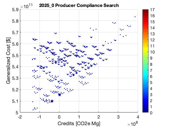 |
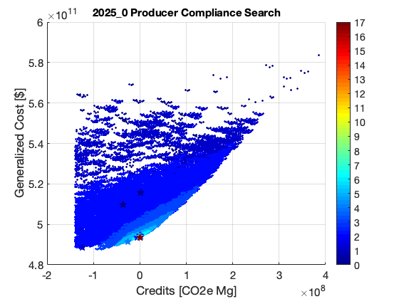 |
Fig. 4.14 Initial compliance search (2025_0)
Fig. 4.15 is another view of the same search, with greater magnification around the selected production option and surrounding options which were not selected.
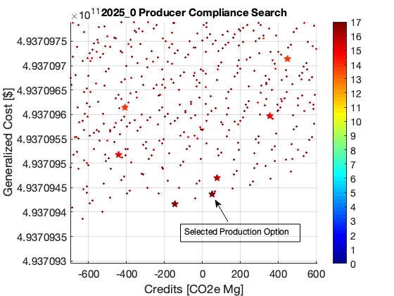
Fig. 4.15 Zoom in on producer’s initial compliance selection (2025_0)
‘Producer-Consumer’ Iteration: Market Shares and Pricing
After a purely cost-minimizing option is selected in the initial compliance search, the Producer Module provides the vehicle attributes and prices, at the market class level, for consideration by the Consumer Module. Within a given Producer-Consumer iteration loop, the vehicle design options are fixed. The search for a solution is based on consideration of various market class share and pricing options. Criteria for convergence include 1) the percent change in average total price, and 2) the difference in the producer and consumer market shares. To achieve convergence, both of these metrics must be close to zero, within the specified tolerance.
Demo example: Consumer-Producer iteration
Within a single Producer-Consumer iteration loop, vehicle designs are fixed, but pricing and market class shares vary. Fig. 4.16 shows the various components of the first Producer-Consumer iteration loop for 2025 in the demo example (Context A, no action policy alternative.)
The upper left panel shows the range of producer cross-subsidy price multiplier options. The full range of multipliers in the 0th sub-iteration are dark blue points, which then narrow in range over eight sub-iterations. The final range of multipliers is shown by the red points.
In the upper right panel, those same pricing options are shown in terms of absolute prices. While the multipliers applied to hauling and non-hauling vehicles cover a similar range of values, the lower absolute prices for non-hauling vehicles results in a range of prices that is somewhat narrower than the range for hauling vehicles.
The two convergence criteria are illustrated in the bottom two panels of Fig. 4.16 (share delta for hauling BEVs in the lower left panel, and average total price delta in the lower right panel.) In this Producer-Consumer iteration, the market class shares offered by the producer do not converge with the shares demanded by the consumer over the range of cross-subsidy pricing options available. This is visible in the lower left panel, since the 0.4% share delta value in the final sub-iteration does not meet the convergence criteria. If convergence had been achieved, the iteration process of this analysis year would be complete, and the produced vehicles would be finalized. Otherwise, the iteration will proceed, with a new consideration of vehicle design options offered by the Producer Module.
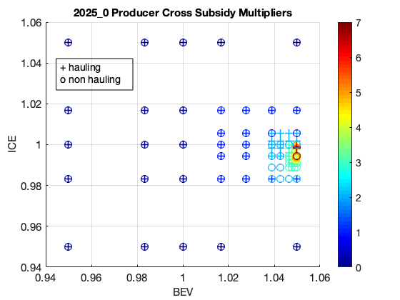 |
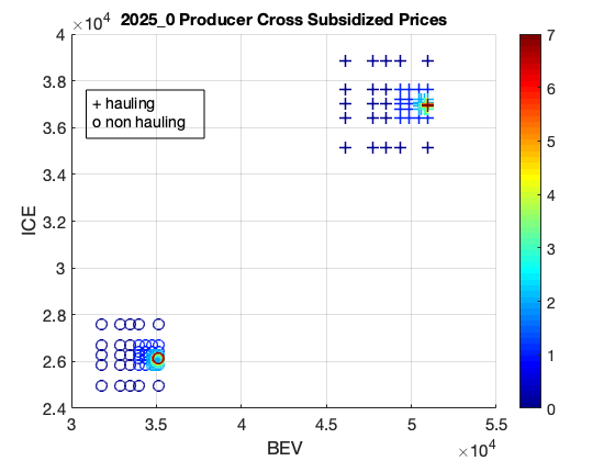 |
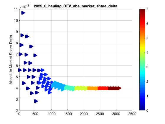 |
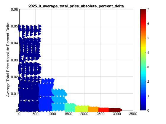 |
Fig. 4.16 Initial Producer-Consumer iteration (2025_0)
Repeat Iteration of ‘Producer-Policy’ and ‘Producer-Consumer’
If the prior round of iterations is unable to find a converged solution, the process will continue by repeating a series of Producer-Policy compliance searches and Producer-Consumer market share and pricing searches. The process is the same as in the initial iteration, with one exception: that the Producer-Policy compliance search will use the market shares from the prior iteration’s Producer-Consumer search.
These iterations are repeated until the market class share and average total price convergence criteria are met, and the compliance search is complete. Alternatively, if the number of Producer-Consumer iterations exceeds the set limit, then the sales and market shares from the last iteration are used. In this case, any deviation from the Producer’s strategic compliance target in that analysis year must be made up for through the use of banked credits. Finally, the produced vehicles are logged for consideration in the Consumer Module’s vehicle stock and use submodules, and in the Effects Module.
Demo example: First iteration beyond initial Producer-Policy and Producer-Consumer iterations
Fig. 4.17 shows the points considered in the compliance search in the first iteration (2025_1) following the initial iteration(2025_0). Similar to the initial iteration, each point represents a compliance option that is the result of a unique combination of candidate vehicle design choices and market class shares. Note that compared to Fig. 4.14, the points in Fig. 4.17 are more sparse since the market shares in this iteration have been constrained to the shares selected in the prior Producer-Consumer iteration.
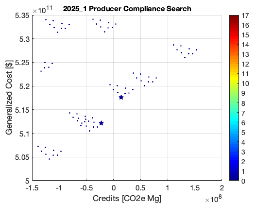 |
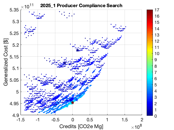 |
Fig. 4.17 Compliance search iteration (2025_1) following initial iteration (2025_0)
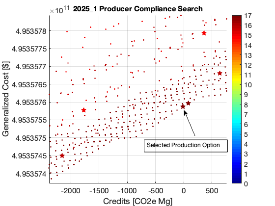
Fig. 4.18 Zoom in on producer’s compliance selection (iteration 2025_1)
Fig. 4.19 is similar to Fig. 4.16, and represents the Producer-Consumer pricing and market class share search in a subsequent round of iteration, after the producer has revised the vehicle design options. Unlike the initial iteration, the range of cross-subsidy pricing flexibility is now sufficient to allow the convergence criteria to be met, as shown in the lower left and lower right panels.
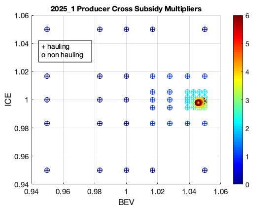 |
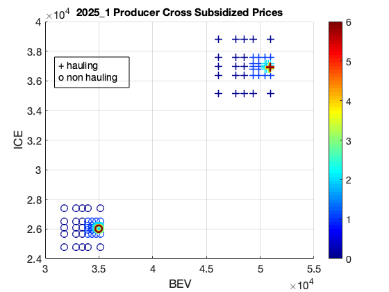 |
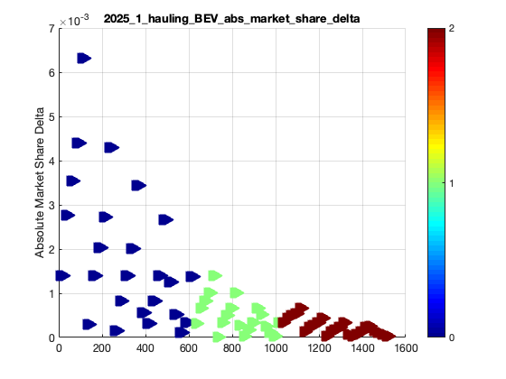 |
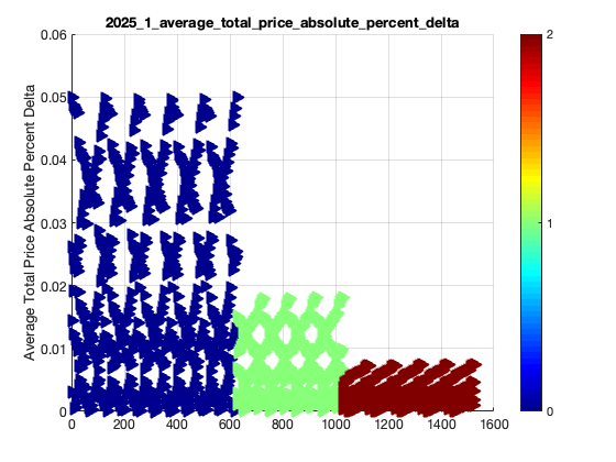 |
Fig. 4.19 Producer-Consumer iteration (2025_1) beyond initial iteration (2025_0)
4.6. Effects Module
In its primary function as a regulatory support tool, OMEGA’s modeled outputs are intended to inform the type of benefit-cost analyses used in EPA rulemakings and other analyses. We would likely use many of OMEGA’s outputs directly in the analysis for a regulatory action. In other cases, OMEGA produces values that might help inform other models like MOVES. The scope of OMEGA’s effects modeling includes estimating both monetized or cost effects and physical effects. The Effects Module builds on the outputs of the Consumer and Producer modules along with the analysis context inputs as shown in Fig. 4.20.
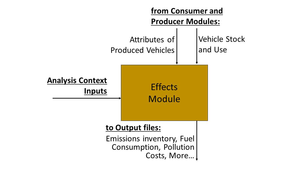
Fig. 4.20 Overview of the Effects Module
- Key examples of physical effects that OMEGA will estimate:
- Stock of registered vehicles, along with key attributes
- VMT of registered vehicles
- Tailpipe GHG and criteria pollutant emissions
- Upstream (refinery, power sector) GHG and criteria pollutant emissions
- Key examples of monetized effects that OMEGA will estimate:
- Vehicle production costs
- Vehicle ownership and operation costs, including fuel and maintenance
- Other consumer effects
- Impacts of criteria air pollutants
- Impacts of greenhouse gas pollutants
- Congestion, noise, and safety costs
The Effects Module generates: physical effects, cost effects, safety effects, benefits and social effects. In general, the cost effects and benefits output files build upon the physical effects output file in conjunction with several of the context input files. Those context input files are the cost factor and emission rate input files. For example, the benefits file would present CO2-related benefits as the CO2 cost factor (a social cost of carbon per metric ton value set in the input file) multiplied by the emission impacts of CO2 (or other GHG) calculated using physical effects. Similarly, fuel costs would be calculated as fuel prices (dollars/gallon as provided in the input file) multiplied by gallons consumed as presented in the physical effects file.
One attribute appears in both the cost effects and the benefits files. That attribute is the drive value which is the economic value of the increased owner/operator surplus provided by added driving and is estimated as one half of the product of the decline in vehicle operating costs per vehicle-mile and the resulting increase in the annual number of miles driven via the rebound effect, plus the cost of driving those round miles. Since the drive value is calculated using a change in operating costs, the new operating costs must be compared to another operating cost. Drive value is calculated as a cost and presented in the cost effects file as the drive surplus plus the fuel costs associated with driving any rebound miles. Drive value is then calculated as a benefit by calculating the the drive value cost in an action scenario relative to the no-action scenario. If the drive value cost is greater in the action scenario, a positive drive value benefit will be the result while a lower drive value cost in the action scenario would represent a negative benefit, or disbenefit.
Importantly, the cost factor inputs (as OMEGA calls them) have been generated using several discount rates. The values calculated using each of the different discount rates should not be added to one another. In other words, PM costs calculated using a 3 percent discount rate and a 7 percent discount rate should never be added together. Similarly, climate costs calculated using a 3 percent discount rate and a 2.5 percent discount rate should never be added. This does not necessarily hold true when adding criteria air pollutant costs and climate costs when it is acceptable to add costs using different discount rates. Lastly, when discounting future values, the same discount rate must be used as was used in generating the cost factors.
The default effects files are annual summary results by calendar year, regulatory class and fuel type. If desired, vehicle-level output files can be selected via the runtime_options.csv file that controls the effects. The vehicle-level output files can be very large depending on the number of vehicles, length of vehicle life and number of calendar years included in the run. Files can be saved in a compressed ‘parquet’ format for use with Python’s pandas library to minimize file sizes.
4.6.1. Physical Effects Calculations
Physical effects are calculated at the vehicle level for all calendar years included in the analysis. Vehicle_ID and VMT driven by the given vehicle are pulled from the VehicleAnnualData class. Vehicle attributes are pulled from VehicleFinal class. Fuel attributes are pulled from the OnroadFuel class which draws them from the onroad_fuels input file.
4.6.2. Fuel Consumption
Liquid fuel consumption and electricity consumption are calculated for a given Vehicle ID as:
Liquid fuel consumption
Where:
- \(VMT_{liquid fuel}=VMT * FuelShare_{liquid fuel}\)
- \((CO_{2} grams/mile)_{onroad, direct}\) is calculated within OMEGA and accounts for any credits that do not improve fuel consumption and test-to-onroad gaps
- \((CO_{2} grams/gallon)\) is the \(CO_{2}\) content of the in-use, or retail, fuel
- \(TransmissionEfficiency\) is the efficiency of liquid fuel transmission as set by the user
Electricity consumption
Where:
- \(VMT_{electricity}=VMT * FuelShare_{electricity}\)
- \((kWh/mile)_{onroad, direct}\) is calculated within OMEGA and accounts for any credits that do not improve fuel consumption and test-to-onroad gaps
- \(TransmissionEfficiency\) is the efficiency of the power grid as set by the user
Note
Multi-fuel vehicle fuel consumption
Multi-fuel vehicles consume both electricity and liquid fuel. Consumption of both is calculated for such vehicles and emission effects such as upstream and tailpipe emissions are calculated uniquely for both fuels.
4.6.3. Emission Inventories
Emission inventories are calculated for a given Vehicle ID as:
Vehicle Exhaust Criteria Emissions (except for SO2)
Where:
- \(Pollutant\) would be any of the criteria air pollutants such as VOC, PM2.5, NOx, etc., with the exception of \(SO_{2}\)
- \(VMT_{liquid fuel}=VMT * FuelShare_{liquid fuel}\)
- \((grams/mile)_{Pollutant}\) is an emission rate from the vehicle emission rates input file
- \(grams/US ton\) = 907,185
Vehicle Exhaust SO2
Where:
- \(FuelConsumption_{liquid fuel}\) is calculated by equation (4.4)
- \((grams/gallon)_{SO_{2}}\) is the \(SO_{2}\) emission rate from the emission rates input file
- \(grams/US ton\) = 907,185
Vehicle Exhaust CH4 and N2O Emissions
Where:
- \(Pollutant\) would be either \(CH_{4}\) or \(N_{2}O\)
- \(VMT_{liquid fuel}=VMT * FuelShare_{liquid fuel}\)
- \((grams/mile)_{Pollutant}\) is an emission rate from the emission rates input file
- \(grams/Metric ton\) = 1,000,000
Vehicle Exhaust CO2 Emissions
Where:
- \(VMT_{liquid fuel}=VMT * FuelShare_{liquid fuel}\)
- \((CO_{2} grams/mile)_{onroad, direct}\) is calculated within OMEGA and accounts for any credits that do not improve fuel consumption and test-to-onroad gaps
- \(grams/Metric ton\) = 1,000,000
Vehicle Brake Wear Criteria Emissions
Where:
- \(Pollutant\) would be any of the criteria air pollutants such as VOC, PM2.5, NOx, etc.
- \((grams/mile)_{Pollutant}\) is an emission rate from the vehicle emission rates input file
- \(grams/US ton\) = 907,185
Vehicle Tire Wear Criteria Emissions
Where:
- \(Pollutant\) would be any of the criteria air pollutants such as VOC, PM2.5, NOx, etc.
- \((grams/mile)_{Pollutant}\) is an emission rate from the vehicle emission rates input file
- \(grams/US ton\) = 907,185
Vehicle Evaporative Criteria Emissions
Where:
- \(FuelConsumption_{liquid fuel}\) is calculated by equation (4.4)
- \((grams/gallon)_{Pollutant}\) is the \(Pollutant\) emission rate from the emission rates input file
- \(grams/US ton\) = 907,185
Upstream Criteria Emissions
Where:
- \(Pollutant\) would be any of the criteria air pollutants such as VOC, PM2.5, NOx, etc.
- \(FC_{kWh}\) is \(FuelConsumption_{kWh}\) calculated by equation (4.5)
- \((grams/kWh)_{Pollutant, EGU}\) is the Electricity Generating Unit (or Power Sector) emission factor for the given Pollutant
- \(FC_{gallons}\) is \(FuelConsumption_{gallons}\) calculated by equation (4.4)
- \((grams/gallon)_{Pollutant, Refinery}\) is the Refinery emission rate for the given pollutant
- \(grams/US ton\) = 907,185
Upstream GHG Emissions
Where:
- \(Pollutant\) would be any of the GHGs such as CO2, CH4, N2O
- \(FC_{kWh}\) is \(FuelConsumption_{kWh}\) calculated by equation (4.5)
- \((grams/kWh)_{Pollutant, EGU}\) is the Electricity Generating Unit (or Power Sector) emission factor for the given Pollutant
- \(FC_{gallons}\) is \(FuelConsumption_{gallons}\) calculated by equation (4.4)
- \((grams/gallon)_{Pollutant, Refinery}\) is the Refinery emission rate for the given pollutant
- \(grams/Metric ton\) = 1,000,000
Total Criteria Emissions
Where:
- \(ExhaustEmission_{Pollutant, tons}\) is calculated by the applicable exhaust emission equation
- \(BrakeEmissions_{Pollutant, tons}\) is calculated by (4.10)
- \(TireEmissions_{Pollutant, tons}\) is calculated by (4.11)
- \(EvaporativeEmissions_{Pollutant, tons}\) is calculated by (4.12)
Where:
- \(VehicleEmissions_{Pollutant, US tons}\) is calculated by equation (4.15)
- \(UpstreamEmissions_{Pollutant, US tons}\) is calculated by equation (4.13)
Total GHG Emissions
Where:
4.6.4. Cost Effects Calculations
Cost effects are calculated at the vehicle level for all calendar years included in the analysis and for, primarily, the physical effects described above.
4.6.5. Benefits Calculations
Benefits are calculated at the fleet level by calendar year and are calculated based on the changes in physical effects relative to the no-action scenario specified in the batch settings input file for the effects run.
5. User Guide
5.1. OMEGA Model
The primary input to OMEGA is the batch definition file which contains rows for each user input required to define a simulation session or group of sessions.
The line-by-line documentation of the batch definition file is available at omega_model/omega_batch.py and won’t be repeated here.
Batch definition inputs can be scalar values or input file paths (relative to the location of the batch file and/or absolute).
Several of the input files may dynamically load user-definable modules at runtime. These files are indicated as user_definable in the table below. User-definable inputs and modules are loaded by interpreting the input file input_template_name: field. For example, if the input template name of a user-definable input is consumer.market_classes then the Python module omega_model/consumer/market_classes.py will be used to load the rest of the input file, which may contain an arbitrary format known to the module. The process of creating user-definable modules is a topic for developers.
Below is a table with links to the modules that load the files and their documentation of the input file formats.
- Batch Input Files and Loaders
- Simulation Context
- The context inputs apply to all sessions within a batch. Multiple batch files must be defined to run multiple contexts.
- Simulation Sessions
- The Reference Session
- The batch file must define at least one simulation session, known as the reference session, which is the left-most session in the batch definition file. The reference session should align with the provided context inputs. For example, if the context fuel price and new vehicle market data are from AEO, then the policy inputs of the reference session must be consistent with the assumptions used by AEO to generate the projections. For example, the sales projections take into account ghg and fuel economy policies in force or projected at the time and the policy inputs used for the reference session should be consistent with those. It would be inconsistent to assume the same sales for a different ghg/fuel economy policy.
- Policy Alternative Sessions
- Optionally, one or more alternative policy sessions may be defined in subsequent columns. Typically these would be various policies under evaluation via OMEGA or perhaps a single policy with various alternative inputs or assumptions.
- OMEGA Batch Command Line Interface
- The batch process can be initiated from the OMEGA GUI or from the command line by running
omega_batch.pydirectly, as in:
>>python omega_model/omega_batch.py --bundle_path path/to/my/bundle_folder --batch_file path/to/my/batch_file.csv

or

>>python omega_model/omega_batch.py --bundle_path path/to/my/bundle_folder --ui_batch_file
In fact, the GUI can be thought of as a wrapper to a command line call to omega_batch.py. The paths supplied to the GUI fill in the --bundle_path and --batch_file arguments.
Typical Command Line Usage (not all available command-line options shown)
usage: omega_batch.py
        [-h] [--bundle_path BUNDLE_PATH] [--batch_file BATCH_FILE]  [--ui_batch_file]
        [--session_num SESSION_NUM] [--analysis_final_year ANALYSIS_FINAL_YEAR]
        [--verbose] [--show_figures]

Run OMEGA batch simulation

optional arguments:
  -h, --help            show this help message and exit

  --bundle_path BUNDLE_PATH
                        Path to bundle folder

  --batch_file BATCH_FILE
                        Path to batch definition file

  --ui_batch_file
                        Select batch file from dialog box

  --session_num SESSION_NUM
                        ID # of session to run from batch

  --analysis_final_year ANALYSIS_FINAL_YEAR
                        Override analysis final year

  --verbose             Enable verbose omega_batch messages
Other command line arguments are available, mostly associated with parallel processing options and implementation or code development. The full list of arguments can be viewed as follows:
>>python omega_model/omega_batch.py

or

>>python omega_model/omega_batch.py -h

or

>>python omega_model/omega_batch.py --help
- Selecting Sessions to Run
- Sessions can be enabled or disabled within the batch file by setting the
Enable Sessionfield toTRUEorFALSE, respectively. Alternatively, the--session_numargument can be passed toomega_batch. The reference session is session number0. The reference session cannot be disabled, regardless of theEnable Sessionfield value, as it generates reference vehicle prices that the other sessions require in order to calculate overall vehicle sales. - Understanding the Batch Process
The first step in the batch process is to copy the complete source code to the
bundlefolder (in theomega_modeldirectory, or as specified by the user via the--bundle_pathargument) and to create subfolders for each active session. Within each session folder will be aninfolder (and anoutfolder will be created when the session runs). The bundle folder contains the original batch definition file as well as a timestamped batch definition file that is actually run. The timestamped file has the original batch settings with new session input file paths relative to the bundle. The bundle folder contains arequirements.txtfile for reference. When running from source code the requirements file indicates the version of Python used to run the batch and contains the list of installed Python packages and their versions at the time, e.g.python_3_8_10_requirements.txt. When running from the executable the contents of theGUI_requirements.txtfile indicates the version number of the GUI.The batch itself and each session will have a log file indicating the progress and success or failure of the process. The batch log file is named
batch_logfile.txtand exists at the top of the bundle folder. Session logs have the prefixo2log_and are located in each session’soutfolder.If a session completes successfully, the session folder is renamed and prepended with an underscore,
_. Failed session folders are prepended with#FAIL_. In this way the session status can be monitored by observing the folder names as the batch runs.Since the bundle folder contains the source code and all inputs for every session it is possible to re-run a batch, or part of a batch, at a later time and reproduce the results if desired. To do so, remove any session folder prefixes and use
omega_batch.pyto re-run the timestamped batch file, while supplying the--no_bundleand--no_validatearguments, since the batch has already been bundled. As in:
>>python path/to/my/bundle_folder/omega_model/omega_batch.py --batch_file path/to/my/bundle_folder/YYYY_MM_DD_hh_mm_ss_batch.csv --no_bundle --no_validate
5.2. OMEGA Effects
The primary inputs to the OMEGA effects calculator are the OMEGA Model’s vehicles and vehicle annual data output files for sessions of interest. For the Effects calculator to find these necessary OMEGA Model output files, the user must provide to the Effects calculator the path where they can be found. This is done via the “batch_settings_effects” input file. Assuming the user has run the OMEGA Model and has the bundled results saved to an accessible directory, then the batch_settings_effects file should provide the full system path to that directory.
Importantly, the batch_settings_effects file must also provide a session name associated with each session for which effects are to be calculated. The session name must be consistent with the session name used in the OMEGA Model run. These session names also need to include a context session name, a no action session name and at least one action session name. These are needed to calculate the effects properly since the context session serves to calculate fleet vehicle miles traveled (VMT) and fleet fuel costs per mile from which any VMT rebound effects in subsequent sessions can be calculated.
The OMEGA effects calculator will look for several necessary files within “in” folder of the context session folder contained within the bundled OMEGA Model results (i.e., the user need not specify these files in the batch_settings_effects file). In particular, the OMEGA effects calculator will look for and find the context fuel prices, price deflator files used to adjust all monetized values into a common valuation, an onroad fuels file, an onroad vehicle calculations file, an annual VMT file, and a reregistration file.
In addition to the context session, a no action and action session are required because some of the effects calculations are meant to calculate impacts of a policy action relative to a no action, or business as usual, policy. In particular, the benefits calculations can only be done by first calculating physical effects of the action policy relative to the no action policy since benefits do not exist, within OMEGA, absent a policy change.
The other inputs to the OMEGA effects calculator are those associated with: vehicle, EGU and refinery emission rates; cost factors, or $/ton, factors associated with criteria air pollutants, GHG emissions, energy security impacts, crashes, congestion, noise, vehicle repair, vehicle maintenance, fuel prices, etc. All of these input files must be provided by the user via the batch_settings_effects file.
Below is a table describing the entries needed in the batch_settings_effects file. User entries are to be made in the
value or full_path columns of the batch_settings_effects file.
- Batch Input Files and Loaders
parameter session_policy description RUNTIME OPTIONS Run ID all enter valuefor the run identifier for your output folder name or blank for default (default is omega_effects)Save Path all enter full pathof the folder to which to save results but do not include unique run identifiersSave Input Files all enter valueas True to save input files to your results folder or False to save space and not do soSave Context Fuel Cost per Mile File all enter valueas True or False and note that these files can be large especially in CSV formatSave Vehicle-Level Safety Effects Files all enter valueas True or False and note that these files can be large especially in CSV formatSave Vehicle-Level Physical Effects Files all enter valueas True or False and note that these files can be large especially in CSV formatSave Vehicle-Level Cost Effects Files all enter valueas True or False and note that these files can be large especially in CSV formatFormat for Vehicle-Level Output Files all enter valueas ‘csv’ for large Excel-readable files or ‘parquet’ for compressed files usable in PandasBATCH SETTINGS batch_folder all enter full_pathof the folder containing OMEGA Model run resultsVehicles File Base Year all enter valueconsistent with the OMEGA Model runAnalysis Final Year all enter value<= the value used in the OMEGA Model runCost Accrual all enter valueas start-of-year or end-of-year - this entry impacts the discounting of costs and benefitsDiscount Values to Year all enter valueto which costs and benefits will be discountedAnalysis Dollar Basis all enter valueconsistent with the OMEGA Model runBatch Analysis Context Settings Context Name all enter valueof the AEO report (e.g. AEO2021) used in the OMEGA Model runContext Case all enter valueof the AEO case (e.g. Reference case) used in the OMEGA Model runVMT Rebound Rate ICE all enter valuefor ICE rebound (e.g. -0.1)VMT Rebound Rate BEV all enter valuefor BEV reboundSC-GHG in Net Benefits all enter valueas ‘global’ or ‘domestic’ or ‘both’ (note that both global and domestic benefits are calculatedthis only impacts net benefits)” Maintenance Costs File all enter full_pathof maintenance costs file in CSV formatRepair Costs File all enter full_pathof repair costs file in CSV formatRefueling Costs File all enter full_pathof refueling costs file in CSV format (i.e. the cost of time spent refueling)General Inputs for Effects File all enter full_pathof general inputs for effects file in CSV formatContext Criteria Cost Factors File all enter full_pathof criteria air pollutant $/ton factors file in CSV formatContext SCC Cost Factors File all enter full_pathof social cost of GHG $/ton factors file in CSV formatContext Energy Security Cost Factors File all enter full_pathof energy security $/barrel file in CSV formatContext Congestion-Noise Cost Factors File all enter full_pathof crashes & congestion & noise costs file in CSV formatContext Legacy Fleet File all enter full_pathof legacy fleet file in CSV formatSession Name context enter valueof the context session name (e.g. SAFE or HDP2_noIRA)Context Stock and VMT File context enter full_pathof stock and VMT file file in CSV formatSession Name no_action enter valueof the no action session name (e.g. NTR or HDP2)Context Powersector Emission Rates File no_action enter full_pathof EGU emission rates file in CSV formatContext Refinery Emission Rates File no_action enter full_pathof refinery emission rates file in CSV formatContext Refinery Emission Factors File no_action leave blank - use is not recommended Context Vehicle Emission Rates File no_action enter full_pathof vehicle emission rates file in CSV formatContext Safety Values File no_action enter full_pathof safety values file in CSV formatContext Fatality Rates File no_action enter full_pathof fatality rates file in CSV formatSession Name action_1 enter valueof the first action or policy session name (e.g. Proposal)Context Powersector Emission Rates File action_1 enter full_pathwhich may be the same as used for the no action sessionContext Refinery Emission Rates File action_1 enter full_pathwhich may be the same as used for the no action sessionContext Refinery Emission Factors File action_1 enter full_pathwhich may be the same as used for the no action sessionContext Vehicle Emission Rates File action_1 enter full_pathwhich may be the same as used for the no action sessionContext Safety Values File action_1 enter full_pathwhich may be the same as used for the no action sessionContext Fatality Rates File action_1 enter full_pathwhich may be the same as used for the no action session
5.2.1. Runtime Options
The effects results will be saved to a folder specified in the save_path full_path entry (e.g. “c:/omega/effects”). In that save_path folder,
a folder will be auto generated and will have the same name as the OMEGA Model batch for which effects are being calculated.
Within that batch folder, a run results folder will be auto generated whose name will consist of a date and timestamp associated with
the time of the OMEGA effects calculator run along with the run ID to assist in keeping track of different runs and ensuring that nothing is
overwritten by future runs. As a result, you might find your results saved to a folder named something like
“c:/omega/effects/ld_omega_model_batch/20230504_090000_omega_effects” for a run done on May 4, 2023, at 9:00AM.
Note that some effects output files may or may not be desired. The effects are calculated for every vehicle in the fleet in every
year up to and including the Analysis Final Year value. If you run through 2055, this becomes a large number of vehicles and
the vehicle-level output files can become very large (0.5 GB to 1 GB per file). Depending on your machine, you may have trouble
viewing those files let alone conducting analyses of the results (e.g., in Excel or OpenOffice). Saving of these large output files
can be avoided by setting the “Save Vehicle-Level” file value to False. Alternatively, the use can generate those files in
parquet format, which is a compressed file format, to save space. Parquet files are readable by Python’s Pandas library but cannot
be opened directly in a spreadsheet application. Instructions for reading saved parquet files in Pandas are included in the save_file function
of /omega_effects/general/file_id_and_save.py.
5.2.2. Batch Analysis Context Settings
The files specified in the Batch Analysis Context Settings section of the batch_settings_effects file are meant to apply to all sessions in the batch.
5.2.3. Session Settings
Any session can be run in the OMEGA Effects calculator provided those sessions exist in the batch_folder. A value for
the session name must be provided. A session can be ignored by setting the Session Name value to None. A Context Session Name
must be provided and no session meant to be included can have a session name of None.
5.2.4. Emission Rates Files
Note that an action session may require a different emission rate input file than that used for the no action session for, say, vehicle emission rates in the event that the policy impacts vehicle emission rates.
5.2.5. Running the OMEGA Effects Executable
- The OMEGA Effects code, input files and output files can be found on the OMEGA webpage at this link https://www3.epa.gov/otaq/ld/lmdv-nprm-effects-docket.zip
- The OMEGA Effects are not part of the OMEGA Model executable file. The OMEGA Effects can be run using the Python code included in the OMEGA repository at https://github.com/USEPA/EPA_OMEGA_Model or the Python code included in the zip file linked above.
- Alternatively, the OMEGA Effects can be run using a separate executable file (recommended).
- These instructions assume that the executable file is being used to generate the OMEGA Effects.
- Place the executable file in your preferred location on your local machine.
- Place the associated “effects_inputs” folder and its contents in your preferred location on your local machine. This folder is available on request to omega_support@epa.gov.
- In the effects_inputs folder, find 2 batch settings files: one for light-duty (batch_settings_effects_ld.csv) and one for medium-duty (batch_settings_effects_md.csv).
- In cell B3 of the batch settings file, enter a run ID if desired (e.g., NPRM, test, etc.). This run ID will be included as part of the output folder name. The default value is omega_effects.
- In cell D4, enter the path of the save folder (e.g., “C:/omega/effects”). The output folder will be saved to this folder. The output folder will be named using other entries in the batch file and the run ID set in step 8.
- Other options in Column B can be set to TRUE or FALSE, but please read the notes associated with each.
- In cell D12 of the batch settings file, enter the full path to the folder that contains your OMEGA compliance run results. This is important since the OMEGA Effects will look to this folder to find the needed vehicles.csv and vehicle_annual_data.csv files generated for each session in your OMEGA compliance run.
- Most values in column C can be left as is. There must be a context session name in cell C34. If your context session name is different, then set cell C34 accordingly. The same is true of subsequent session names in column C. If you do not want your effects outputs to include a session that exists in your OMEGA compliance run folder, simply set the session name to None.
- Remaining entries in Column D should then point to the “effects_inputs” folder on your local machine. Filenames can probably be left as is unless you are using files with different names.
- After setting up the batch settings file, be sure to save it as a CSV file (not Excel).
- Double click the executable file.
- The executable should launch. Be patient. After several seconds, a file dialog window should open asking for the batch settings file. Navigate to the batch settings file you saved in step 14, select it, and click open. The executable should now run using the settings in your batch settings file.
6. Developer Guide
This Developer Guide will assist those interested in the latest (pre-release) version of OMEGA available from source code. This guide assumes some familiarity with Python programming and development, but also attempts to point newcomers in the right direction where possible.
6.1. Github Repository
The development version of OMEGA is available in the developer branch of the EPA_OMEGA_Model GitHub repository:
https://github.com/USEPA/EPA_OMEGA_Model
The developer branch contains in-development, pre-release code, subject to change without notice and no guarantees as to stability at any given point in time. Features may be added or removed and may or may not be used for future rulemakings.
Releases will be available on separate branches that contain only the particular release in question.
The developer branch can be accessed via .zip file directly (https://github.com/USEPA/EPA_OMEGA_Model/archive/refs/heads/developer.zip), via GitHub-integrated development environments or via GitHub command-line calls (e.g. gh repo clone USEPA/EPA_OMEGA_Model).
The OMEGA development team uses PyCharm Community Edition to write and debug code, but any Python development environment may be used.
6.2. Setup
After downloading the source code (via .zip file or cloning the repository), it is necessary to install Python and various required Python packages.
6.2.1. Python
The latest versions of Python are available at https://www.python.org/downloads/
OMEGA has been developed with Python versions 3.7.1 (the minimum required version) thru 3.9.13 and has not been tested with version 3.10 or higher. If you already have Python installed, there is probably no reason to update to a newer version unless one of the required packages is not compatible with your Python version and hardware platform.
The recommended practice is to run the source code in a virtual environment, which may be set up manually or via the IDE. The virtual environment isolates the installation of OMEGA-required Python packages from whatever packages may have already been installed at the system level. This allows a ‘clean’ installation that can guarantee no known conflicts between packages.
6.2.2. Required Packages
In addition to Python, OMEGA requires several publicly available Python packages in order to run. These are detailed in the requirements.txt file.
6.2.2.1. Simple Install
The simplest way to install the packages is to use pip, the package installer for Python. Sometimes there is an updated version of pip available. The command-line code below updates pip and installs the packages detailed in requirements.txt.
python -m pip install --upgrade pip setuptools
pip install -r requirements.txt
6.2.2.2. conda / pip Install
Many of the most popular Python packages include pre-compiled versions that are intended for specific hardware. However, depending on your development environment (ARM-based Mac, for example) it may be useful (or necessary) to get some of the pre-compiled packages from other sources, such as Anaconda / Conda. A lightweight conda install is available via miniforge. The full Anaconda installation is quite large, so if it is not already installed then it is recommended to use something like miniforge instead.
This more advanced installation method has two steps
- install available pre-compiled packages via
conda- install any remaining packages via
pip
conda install --file requirements-conda.txt
pip install -r requirements.txt
requirements-conda.txt may need to be tailored to the developer’s specific operating system and hardware but should serve as a good starting point.
6.2.3. Running From Source Code
There are at least four common ways to run OMEGA:
- from the executable GUI (see Getting Started and Running the Demo Example using the Graphical User Interface (GUI))
- from source at the command line as a single (default) session via
omega_model.omega- from source at the command line as a GUI via
omega_gui.omega_gui- from source at the command line as a batch via
omega_model.omega_batch(See also Omega Batch Command Line Interface)
To run the default session directly from source at the command line from the project top-level folder:
python omega_model/omega.py
Will produce output such as:
loading omega version X.Y.Z
importing XXX.py

...

Initializing OMEGA Quick Test:
importing XYZ.py

...

Running OMEGA Quick Test:

Running OMEGA Quick Test Pass 0: Manufacturer=consolidated_OEM
Running OMEGA Quick Test:  Year=2020  Iteration=0 consolidated_OEM
Running OMEGA Quick Test:  Year=2020  Iteration=1 consolidated_OEM
Running OMEGA Quick Test:  Year=2020  Iteration=2 consolidated_OEM
Running OMEGA Quick Test:  Year=2021  Iteration=0 consolidated_OEM
Running OMEGA Quick Test:  Year=2021  Iteration=1 consolidated_OEM
Running OMEGA Quick Test:  Year=2021  Iteration=2 consolidated_OEM

Session ended at 2023-04-05 11:38:00
Session elapsed time 120.56 seconds
The primary use case for running omega.py directly is just to confirm the installation or perhaps when it’s simpler to debug code without the overhead of the batch process.
To run the gui directly from source at the command line from the project top-level folder:
python omega_gui/omega_gui.py
For all other development use cases it is recommended to run omega_batch.py as shown in the User Guide under Omega Batch Command Line Interface
7. Code Details
7.1. omega_effects package
OMEGA effects post-processing subpackage.
CODE
7.1.1. Subpackages
7.1.1.1. omega_effects.consumer package
OMEGA effects code consumer subpackage.
CODE
7.1.1.1.1. Submodules
7.1.1.1.2. omega_effects.consumer.annual_vmt_fixed_by_age module
Routines to load and provide access to annual vehicle miles travelled (VMT) by market class and age.
The data represents a fixed VMT schedule by age.
INPUT FILE FORMAT
The file format consists of a one-row template header followed by a one-row data header and subsequent data rows. The template header uses a dynamic format.
The data represents the re-registered proportion of vehicles by calendar year, age and market class.
- File Type
- comma-separated values (CSV)
- Template Header
input_template_name: [module_name]input_template_version: [template_version]- Sample Header
input_template_name: consumer.annual_vmt_fixed_by_age input_template_version: 0.2 - Sample Data Columns
start_year age market_class_id annual_vmt 2019 0 non_hauling.BEV 14699.55515 2019 1 non_hauling.BEV 14251.70373 2019 2 non_hauling.BEV 14025.35397 2019 0 hauling.ICE 15973.88982 2019 1 hauling.ICE 15404.1216 2019 2 hauling.ICE 14840.93011
| start_year: | Start year of annual VMT data, values apply until the next available start year |
|---|---|
| age: | Vehicle age, in years |
| market_class_id: | |
| Vehicle market class ID, e.g. ‘hauling.ICE’ | |
| annual_vmt: | Vehicle miles travelled per year at the given age for the given market class ID |
CODE
-
class
OnroadVMT¶ Bases:
objectLoads and provides access to annual Vehicle Miles Travelled by calendar year, market class, and age.
-
__init__()¶ Initialize self. See help(type(self)) for accurate signature.
-
get_cumulative_vmt(market_class_id, age)¶ Get cumulative VMT for the given market class id and age.
Parameters: - market_class_id (str) – market class id, e.g. ‘hauling.ICE’
- age (int) – vehicle age in years
Returns: Cumulative VMT for the given market class id and age.
-
get_vmt(calendar_year, market_class_id, age)¶ Get vehicle miles travelled by calendar year, market class and age.
Parameters: - calendar_year (int) – calendar year of the VMT data
- market_class_id (str) – market class id, e.g. ‘hauling.ICE’
- age (int) – vehicle age in years
Returns: (float) Annual vehicle miles travelled.
-
init_from_file(filepath, effects_log)¶ Initialize class data from input file.
Parameters: - filepath – the Path object to the file.
- effects_log – an instance of the EffectsLog class.
Returns: Nothing, but reads the appropriate input file.
-
7.1.1.1.3. omega_effects.consumer.deregionalizer module
OMEGA effects code de-regionalizer module.
Used with ‘zev’ and ‘nonzev’ market classes.
CODE
-
clean_body_styles(df)¶ Parameters: df (DataFrame) – DataFrame containing body_style entries to be made consistent. Returns: DataFrame with body_styles consistent with effects inputs.
-
deregionalize_entries(df, attribute, *args)¶ Parameters: - df (DataFrame) – DataFrame containing region specific values to be deregionalized.
- attribute (str) – the attribute to act on (e.g., ‘market_class_id’, ‘body_style’).
- args (str or strs) – the strings to remove from entries.
Returns: A new DataFrame with region specific data removed.
-
remove_region_entries(df, attribute, attribute_values_to_remove, string_for_removal, *args)¶ Parameters: - df (DataFrame) – DataFrame containing region specific values to be removed.
- attribute (str) – the attribute to act on (e.g., ‘market_class_id’, ‘body_style’).
- attribute_values_to_remove (str) – the string to search on to remove entries (e.g., ‘r1nonzev’, ‘r2zev’).
- string_for_removal (str) – the string to replace while keeping entries (e.g., ‘r1nonzev’, ‘r2zev’).
- args (str or strs) – the attribute values to be deregionalized.
Returns: A new DataFrame with region specific data removed.
7.1.1.1.4. omega_effects.consumer.reregistration_fixed_by_age module
Vehicle re-registration, fixed by age.
INPUT FILE FORMAT
The file format consists of a one-row template header followed by a one-row data header and subsequent data rows. The template header uses a dynamic format.
The data represents the re-registered proportion of vehicles by model year, age and market class.
- File Type
- comma-separated values (CSV)
- Template Header
input_template_name: [module_name]input_template_version: [template_version]- Sample Header
input_template_name: consumer.reregistration_fixed_by_age input_template_version: 0.2 - Sample Data Columns
start_model_year age market_class_id reregistered_proportion 1970 0 non_hauling.BEV 1 1970 1 non_hauling.BEV 0.987841531 1970 2 non_hauling.BEV 0.976587217 1970 0 hauling.ICE 1 1970 1 hauling.ICE 0.977597055 1970 2 hauling.ICE 0.962974697
Data Column Name and Description
| start_model_year: | |
|---|---|
| The start vehicle model year of the re-registration data, values apply until next available start year | |
| age: | Vehicle age, in years |
| market_class_id: | |
| Vehicle market class ID, e.g. ‘hauling.ICE’ | |
| reregistered_proportion: | |
| The fraction of vehicles re-registered, [0..1] | |
CODE
-
class
Reregistration¶ Bases:
objectLoad and provide access to vehicle re-registration data by model year, market class ID and age.
-
__init__()¶ Initialize self. See help(type(self)) for accurate signature.
-
get_reregistered_proportion(model_year, market_class_id, age)¶ Get vehicle re-registered proportion [0..1] by market class and age.
Parameters: - model_year (int) – the model year of the re-registration data
- market_class_id (str) – market class id, e.g. ‘hauling.ICE’
- age (int) – vehicle age in years
Returns: Re-registered proportion [0..1]
-
init_from_file(filepath, effects_log)¶ Initialize class data from input file.
Parameters: - filepath – the Path object to the file.
- effects_log – an instance of the EffectsLog class.
Returns: Nothing, but reads the appropriate input file.
-
7.1.1.2. omega_effects.context package
OMEGA effects code context subpackage.
CODE
7.1.1.2.1. Submodules
7.1.1.2.2. omega_effects.context.context_stock_vmt module
Routines to load and access stock vmt from the analysis context
INPUT FILE FORMAT
The file format consists of a one-row template header followed by a one-row data header and subsequent data rows.
The data represents stock vmt by context case, case id and calendar year.
- File Type
- comma-separated values (CSV)
- Sample Header
input_template_name: context_stock_vmt input_template_version: 0.1 - Sample Data Columns
context_id calendar_year case_id miles stock AEO2022 2021 Reference case 2.76E+12 260088654 AEO2022 2022 Reference case 2.89E+12 261614075 AEO2022 2023 Reference case 2.99E+12 263155182 AEO2022 2024 Reference case 3.03E+12 264624603 AEO2022 2025 Reference case 3.08E+12 266039459 - Data Column Name and Description
context_id: The name of the context source, e.g. ‘AEO2020’, ‘AEO2021’, etc case_id: The name of the case within the context, e.g. ‘Reference Case’, ‘High oil price’, etc calendar_year: The calendar year of the fuel costs miles: The vehicle miles traveled stock: The vehicle stock
CODE
-
class
ContextStockVMT¶ Bases:
objectLoads and provides access to stock vmt from the analysis context
-
__init__()¶ Initialize self. See help(type(self)) for accurate signature.
-
get_context_stock_vmt(calendar_year)¶ Parameters: calendar_year (int) – the calendar year for which stock vmt is sought Returns: The stock and vmt values for the passed calendar year
-
init_from_file(filepath, batch_settings, effects_log)¶ Initialize class data from input file.
Parameters: - filepath – the Path object to the file.
- batch_settings – an instance of the BatchSettings class.
- effects_log – an instance of the EffectsLog class.
Returns: Nothing, but reads the appropriate input file.
-
7.1.1.2.3. omega_effects.context.cpi_price_deflators module
Routines to load CPI price deflators.
Used to convert monetary general to a consistent dollar basis, e.g., in the cost_factors_criteria module.
INPUT FILE FORMAT
The file format consists of a one-row template header followed by a one-row data header and subsequent data rows.
The data represents the price deflator by calendar year.
- File Type
- comma-separated values (CSV)
- Sample Header
input_template_name: context_cpi_price_deflators input_template_version: 0.22 - Sample Data Columns
calendar_year price_deflator 2010 218.056 2011 224.939
Data Column Name and Description
| calendar_year: | Calendar year of the price deflator |
|---|---|
| price_deflator: | CPI price deflator |
CODE
-
class
CPIPriceDeflators¶ Bases:
objectLoads and provides access to CPI price deflators by calendar year.
-
__init__()¶ Initialize self. See help(type(self)) for accurate signature.
-
adjust_dollars(batch_settings, df, effects_log, *args)¶ Parameters: - batch_settings – an instance of the BatchSettings class.
- df (DataFrame) – values to be converted to a consistent dollar basis.
- effects_log – an instance of the EffectsLog class.
- args (str or strs) – The attributes to be converted to a consistent dollar basis.
Returns: The passed DataFrame with args expressed in a consistent dollar basis.
-
get_price_deflator(calendar_year, effects_log)¶ Get the CPI price deflator for the given calendar year.
Parameters: - calendar_year (int) – the calendar year to get the function for
- effects_log – an instance of the EffectsLog class
Returns: The CPI price deflator for the given calendar year.
-
init_from_file(filepath, effects_log)¶ Initialize class data from input file.
Parameters: - filepath – the Path object to the file.
- effects_log – an instance of the EffectsLog class.
Returns: Nothing, but reads the appropriate input file.
-
7.1.1.2.4. omega_effects.context.fuel_prices module
Routines to load and access fuel prices from the analysis context
Context fuel price data includes retail and pre-tax costs in dollars per unit (e.g. $/gallon, $/kWh)
INPUT FILE FORMAT
The file format consists of a one-row template header followed by a one-row data header and subsequent data rows.
The data represents fuel prices by context case, fuel type, and calendar year.
- File Type
- comma-separated values (CSV)
- Sample Header
input_template_name: context_fuel_prices input_template_version: 0.2 - Sample Data Columns
context_id dollar_basis case_id fuel_id calendar_year retail_dollars_per_unit pretax_dollars_per_unit AEO2020 2019 Reference case pump gasoline 2019 2.665601 2.10838 AEO2020 2019 Reference case US electricity 2019 0.12559407 0.10391058 - Data Column Name and Description
context_id: The name of the context source, e.g. ‘AEO2020’, ‘AEO2021’, etc dollar_basis: The dollar basis of the fuel prices in the given AEO version. Note that this dollar basis is converted in-code to ‘analysis_dollar_basis’ using the implicit_price_deflators input file. case_id: The name of the case within the context, e.g. ‘Reference Case’, ‘High oil price’, etc fuel_id: The name of the vehicle in-use fuel, must be in the table loaded by class fuels.Fueland consistent with the base year vehicles file (columnin_use_fuel_id) loaded byclass vehicles.VehicleFinalcalendar_year: The calendar year of the fuel costs retail_dollars_per_unit: Retail dollars per unit pretax_dollars_per_unit: Pre-tax dollars per unit
CODE
-
class
FuelPrice¶ Bases:
objectLoads and provides access to fuel prices from the analysis context
-
__init__()¶ Initialize self. See help(type(self)) for accurate signature.
-
get_fuel_prices(batch_settings, calendar_year, price_types, fuel_id)¶ Get fuel price data for fuel_id in calendar_year
Parameters: - batch_settings – an instance of the BatchSettings class.
- calendar_year (numeric) – calendar year for which to get fuel prices.
- price_types (str, [str1, str2...]) – ContextFuelPrices attributes to get
- fuel_id (str) – fuel ID
Returns: Fuel price or tuple of fuel prices if multiple attributes were requested
Example
pretax_pump_gas_price_dollars_2030 =
ContextFuelPrices.get_fuel_prices(2030, 'pretax_dollars_per_unit', 'pump gasoline')

pump_gas_attributes_2030 =
ContextFuelPrices.get_fuel_prices(2030, ['retail_dollars_per_unit', 'pretax_dollars_per_unit'], 'pump gasoline')
-
init_from_file(filepath, batch_settings, effects_log)¶ Initialize class data from input file.
Parameters: - filepath – the Path object to the file.
- batch_settings – an instance of the BatchSettings class.
- effects_log – an instance of the EffectsLog class.
Returns: Nothing, but reads the appropriate input file.
-
7.1.1.2.5. omega_effects.context.ip_deflators module
Routines to load Implicit Price (IP) deflators.
Used to convert monetary general to a consistent dollar basis, e.g., in the cost_factors_congestion_noise module.
INPUT FILE FORMAT
The file format consists of a one-row template header followed by a one-row data header and subsequent data rows.
The data represents the price deflator by calendar year.
- File Type
- comma-separated values (CSV)
- Sample Header
input_template_name: context_implicit_price_deflators input_template_version: 0.22 - Sample Data Columns
calendar_year price_deflator 2001 79.783 2002 81.026
Data Column Name and Description
| calendar_year: | Calendar year of the price deflator |
|---|---|
| price_deflator: | Implicit price deflator |
CODE
-
class
ImplicitPriceDeflators¶ Bases:
objectLoads and provides access to implicit price deflators by calendar year.
-
__init__()¶ Initialize self. See help(type(self)) for accurate signature.
-
adjust_dollars(batch_settings, df, effects_log, *args)¶ Parameters: - batch_settings – an instance of the BatchSettings class.
- df (DataFrame) – values to be converted to a consistent dollar basis.
- effects_log – an instance of the EffectsLog class.
- args (str or strs) – The attributes to be converted to a consistent dollar basis.
Returns: The passed DataFrame with args expressed in a consistent dollar basis.
-
dollar_adjustment_factor(batch_settings, dollar_basis_input, effects_log)¶ Parameters: - batch_settings – an instance of the BatchSettings class.
- dollar_basis_input (int) – the dollar basis of the cost to be adjusted.
- effects_log – an instance of the EffectsLog class.
Returns: The multiplicative factor that can be applied to a cost in dollar_basis_input to express that value in analysis_dollar_basis.
-
get_price_deflator(calendar_year, effects_log)¶ Get the implicit price deflator for the given calendar year.
Parameters: - calendar_year (int) – the calendar year to get the function for
- effects_log – an instance of the EffectsLog class.
Returns: The implicit price deflator for the given calendar year.
-
init_from_file(filepath, effects_log)¶ Initialize class data from input file.
Parameters: - filepath – the Path object to the file.
- effects_log – an instance of the EffectsLog class.
Returns: Nothing, but reads the appropriate input file.
-
7.1.1.2.6. omega_effects.context.maintenance_cost module
Routines to load Maintenance Cost Inputs.
INPUT FILE FORMAT
The file format consists of a one-row template header followed by a one-row data header and subsequent data rows.
The data represent various inputs for use in maintenance cost calculations.
- File Type
- comma-separated values (CSV)
- Sample Header
input_template_name: maintenance_cost input_template_version: 0.2 - Sample Data Columns
item miles_per_event_ICE miles_per_event_HEV miles_per_event_PHEV miles_per_event_BEV dollars_per_event dollar_basis Engine Oil 7500 7500 9000 65 2019 Oil Filter 7500 7500 9000 20 2019 Tire Rotation 7500 7500 7500 7500 50 2019
Data Column Name and Description
| item: | The maintenance attribute name. |
|---|---|
| miles_per_event_ICE: | |
| The attribute value for ICE vehicles. | |
| miles_per_event_HEV: | |
| The attribute value for HEVs. | |
| miles_per_event_PHEV: | |
| The attribute value for PHEVs. | |
| miles_per_event_BEV: | |
| The attribute value for BEVs. | |
| dollars_per_event: | |
| The cost in US dollars per maintenance event. | |
| dollar_basis: | The dollar basis of values within the table. Values are converted in-code to ‘analysis_dollar_basis’ using the implicit_price_deflators input file. |
CODE
-
class
MaintenanceCost¶ Bases:
objectLoads and provides access to maintenance cost input values for effects calculations.
-
__init__()¶ Initialize self. See help(type(self)) for accurate signature.
-
static
calc_maintenance_cost_per_mile(input_dict)¶ Calc maintenance cost per mile.
Parameters: input_dict – Dictionary of the maintenance cost inputs. Returns: The input_dict with the total maintenance cost per mile added; this cost per mile would be a constant for all miles. Notes
This method is not being used currently in favor of the calc_maintenance_cost_per_mile_curve method within the class.
-
static
calc_maintenance_cost_per_mile_curve(input_df)¶ Parameters: input_df – DataFrame reflecting the maintenance_cost_inputs.csv file with costs updated to analysis_basis_dollars. Returns: - A dictionary of maintenance cost curve coefficients (slope with intercept=0)
- having keys of ‘ICE’, ‘HEV’, ‘PHEV’, ‘BEV’.
Notes
Dividing the cumulative_cost by miles gives a constant cost/mile for every mile. However, costs/mile should be lower early and higher later, so this method determines a triangular area that equates to the cumulative cost. With the slope of that triangular area, a cost/mile at any odometer value can be calculated and the cost of maintenance in any year can then be calculated as that cost/mile multiplied by miles driven in that year.
-
get_maintenance_cost_curve_coefficients(veh_type)¶ Parameters: veh_type (str) – The type of powertrain in the vehicle, e.g., ‘ICE’, ‘BEV’, ‘HEV’, ‘PHEV’ Returns: The maintenance cost curve coefficients for the given veh_type.
-
init_from_file(filepath, batch_settings, effects_log)¶ Initialize class data from input file.
Parameters: - filepath – the Path object to the file.
- batch_settings – an instance of the BatchSettings class.
- effects_log – an instance of the EffectsLog class.
Returns: Nothing, but reads the appropriate input file.
-
7.1.1.2.7. omega_effects.context.onroad_fuels module
Routines to load and retrieve onroad (in-use) fuel attribute data
Fuel data includes a name, units (e.g. gallons, kWh), CO2e g/unit, refuel_efficiency and transmission_efficiency.
See also
vehicles and context_fuel_prices modules, and consumer subpackage
INPUT FILE FORMAT
The file format consists of a one-row template header followed by a one-row data header and subsequent data rows.
The data represents fuel property data for on-road/in-use purposes.
- File Type
- comma-separated values (CSV)
- Sample Header
input_template_name: onroad-fuels input_template_version: 0.1 - Sample Data Columns
fuel_id start_year unit direct_co2e_grams_per_unit refuel_efficiency transmission_efficiency pump gasoline 2020 gallon 8887 1 1 US electricity 2020 kWh 0 0.9 0.935
Data Column Name and Description
| fuel_id: | The Fuel ID, as referenced by the vehicles and context_fuel_prices modules, and consumer subpackage. |
|---|---|
| start_year: | Start year of fuel properties, properties apply until the next available start year |
| unit: | Fuel unit, e.g. ‘gallon’, ‘kWh’ |
| direct_co2e_grams_per_unit: | |
| CO2e emissions per unit when consumed | |
| refuel_efficiency: | |
| Refuel efficiency [0..1], e.g. electrical vehicle charging efficiency | |
| transmission_efficiency: | |
| Fuel transmission efficiency [0..1], e.g. electrical grid efficiency, may also be referred to as “grid loss” | |
CODE
-
class
OnroadFuel¶ Bases:
objectLoads and provides methods to access onroad fuel attribute data.
-
__init__()¶ Initialize self. See help(type(self)) for accurate signature.
-
get_fuel_attribute(calendar_year, in_use_fuel_id, attribute)¶ Parameters: - calendar_year (numeric) – year to get fuel properties in
- in_use_fuel_id (str) – e.g. ‘pump gasoline’)
- attribute (str) – name of attribute to retrieve
Returns: Fuel attribute value for the given year.
Example
carbon_intensity_gasoline =
    OnroadFuel.get_fuel_attribute(2020, 'pump gasoline', 'direct_co2e_grams_per_unit')
-
init_from_file(filepath, effects_log)¶ Initialize class data from input file.
Parameters: - filepath – the Path object to the file.
- effects_log – an instance of the EffectsLog class.
Returns: Nothing, but reads the appropriate input file.
-
7.1.1.2.8. omega_effects.context.powertrain_cost module
Routines to powertrain cost.
INPUT FILE FORMAT
The file format consists of a one-row template header followed by a one-row data header and subsequent data rows. The template header uses a dynamic format.
- File Type
- comma-separated values (CSV)
- Sample Header
input_template_name: powertrain_cost input_template_version: 0.1 {optional_source_data_comment}- Sample Data Columns
powertrain_type item value quantity dollar_basis notes ALL dollars_per_cylinder ((-28.814) * CYL + 726.27) * CYL * MARKUP_ICE 2019 ALL dollars_per_liter ((400) * LITERS) * MARKUP_ICE 2019 ALL gdi ((43.237) * CYL + 97.35) * MARKUP_ICE 2019 BEV battery_offset {“dollars_per_kwh”: {2023: -9 2024: -18 2025: -27 2026: -36 2027: -45 2028: -45 2029: -45 2030: -33.75 2031: -22.50 2032: -11.25 2033: -0}}
Data Column Name and Description
powertrain_type: Vehicle powertrain type, e.g. ‘ICE’, ‘PHEV’, etc item: The name of the powertrain component associated with the cost value value: The component cost value or equation to be evaulated quantity: Component quantity per vehicle, if applicable dollar_basis: The dollar basis year for the cost value, e.g. 2020notes: Optional notes related to the data row
CODE
-
class
PowertrainCost¶ Bases:
objectLoads and provides access to maintenance cost input values for effects calculations.
-
__init__()¶ Initialize self. See help(type(self)) for accurate signature.
-
get_battery_tax_offset(year, battery_kwh)¶ Get battery tax offset.
Parameters: - year (int) – year for which battery tax credit is needed.
- battery_kwh (float) – battery pack capacity in kWh
Returns: The battery tax offset (dollars per kWh credit) for the given year.
-
init_from_file(filepath, effects_log)¶ Initialize class data from input file.
Parameters: - filepath – the Path object to the file.
- effects_log – an instance of the EffectsLog class.
Returns: Nothing, but reads the appropriate input file.
-
7.1.1.2.9. omega_effects.context.refueling_cost module
Routines to load Refueling Cost Inputs.
INPUT FILE FORMAT
The file format consists of a one-row template header followed by a one-row data header and subsequent data rows.
The data represent various inputs for use in refueling cost calculations.
- File Type
- comma-separated values (CSV)
- Sample Header
input_template_name: refueling_cost input_template_version: 0.2 - Sample Data Columns
type item value dollar_basis car miles_to_mid_trip_charge 7840 + -64.4 * range + 0.18 * range ** 2 truck miles_to_mid_trip_charge 6290 + -49.9 * range + 0.135 * range ** 2 suv share_of_miles_charged_mid_trip 0.241 + -0.001 * range + 0.000001 * range ** 2 truck fixed_refueling_minutes 3.5
Data Column Name and Description
| type: | The vehicle type, e.g. ‘car’, ‘suv’, etc |
|---|---|
| item: | The refueling cost curve attribute name |
| value: | Scalar value or expression to be evaluated for cost |
| dollar_basis: | The dollar basis year for the cost value, e.g. 2020 |
CODE
-
class
RefuelingCost¶ Bases:
objectLoads and provides access to refueling cost input values for refueling cost calculations.
-
__init__()¶ Initialize self. See help(type(self)) for accurate signature.
-
calc_bev_refueling_cost_per_mile(vehicle_type, bev_range)¶ Parameters: - vehicle_type (str) – The type of vehicle, e.g., ‘car’, ‘suv’, ‘truck’.
- bev_range (int) – The range (miles) of the BEV on a full charge.
Returns: The refueling cost per mile for the given veh_type.
-
calc_liquid_refueling_cost_per_gallon(vehicle_type)¶ Parameters: vehicle_type (str) – The type of vehicle, e.g., ‘car’, ‘suv’, ‘truck’. Returns: The refueling cost per mile for the given veh_type.
-
init_from_file(filepath, batch_settings, effects_log)¶ Initialize class data from input file.
Parameters: - filepath – the Path object to the file.
- batch_settings – an instance of the BatchSettings class.
- effects_log – an instance of the EffectsLog class.
Returns: Nothing, but reads the appropriate input file.
-
7.1.1.2.10. omega_effects.context.repair_cost module
Routines to load Repair Cost Inputs.
INPUT FILE FORMAT
The file format consists of a one-row template header followed by a one-row data header and subsequent data rows.
The data represent various inputs for use in repair cost calculations.
- File Type
- comma-separated values (CSV)
- Sample Header
input_template_name: repair_cost input_template_version: 0.1 - Sample Data Columns
item value car_multiplier 1 suv_multiplier 0.91 truck_multiplier 0.7 ICE_multiplier 1 HEV_multiplier 0.91
Data Column Name and Description
| item: | The repair cost curve attribute name. |
|---|---|
| value: | The attribute value. |
CODE
-
class
RepairCost¶ Bases:
objectLoads and provides access to repair cost input values for repair cost calculations.
-
__init__()¶ Initialize self. See help(type(self)) for accurate signature.
-
calc_repair_cost_per_mile(veh_cost, pt_type, repair_type, age)¶ Parameters: - veh_cost – (Numeric) The value of the vehicle when sold as new
- pt_type – (str) The powertrain type (ICE, HEV, PHEV, BEV)
- repair_type – (str) The vehicle repair type (car, suv, truck)
- age – (int) The age of the vehicle where age=0 is year 1 in operation.
Returns: A single repair cost per mile for the given vehicle at the given age.
-
init_from_file(filepath, effects_log)¶ Initialize class data from input file.
Parameters: - filepath – the Path object to the file.
- effects_log – an instance of the EffectsLog class.
Returns: Nothing, but reads the appropriate input file.
-
7.1.1.3. omega_effects.effects package
OMEGA effects main subpackage.
CODE
7.1.1.3.1. Submodules
7.1.1.3.2. omega_effects.effects.benefits module
OMEGA effects benefits module.
CODE
-
calc_benefits(batch_settings, annual_physical_effects_df, annual_cost_effects_df, calc_health_effects=False)¶ Parameters: - batch_settings – an instance of the BatchSettings class.
- annual_physical_effects_df (DataFrame) – a DataFrame of physical effects by calendar year, reg class, fuel type.
- annual_cost_effects_df (DataFrame) – a DataFrame of cost effects by calendar year, reg class, fuel type.
- calc_health_effects (bool) – criteria air pollutant (cap) benefits will be calculated if True.
Returns: one of benefits for each action session relative to the no_action session; and one of physical effects for each action session relative to the no_action session.
Return type: Two dictionaries
-
get_cap_cf(batch_settings, calendar_year, source_id)¶ Get criteria cost factors
Parameters: - batch_settings – an instance of the BatchSettings class.
- calendar_year (int) – The calendar year for which criteria cost factors are needed.
- source_id (str) – the pollutant source, e.g., ‘car pump gasoline’, ‘egu’, ‘refinery’
Returns: A list of cost factors as specified in the cost_factors list for the given calendar year.
-
get_energysecurity_cf(batch_settings, calendar_year)¶ Get energy security cost factors
Parameters: - batch_settings – an instance of the BatchSettings class.
- calendar_year – The calendar year for which energy security related factors are needed.
Returns: A list of cost factors as specified in the cost_factors list for the given calendar year.
-
get_scc_cf(batch_settings, calendar_year)¶ Get social cost of carbon cost factors
Parameters: - batch_settings – an instance of the BatchSettings class.
- calendar_year (int) – The calendar year for which social cost of GHG cost factors are needed.
Returns: A list of cost factors as specified in the cost_factors list for the given calendar year.
7.1.1.3.3. omega_effects.effects.context_fuel_cost_per_mile module
Function to calculate fuel costs per mile in the reference session against which rebound effects can be calculated for subsequent sessions.
CODE
-
calc_fuel_cost_per_mile(batch_settings, session_settings)¶ Parameters: - batch_settings – an instance of the BatchSettings class.
- session_settings – an instance of the SessionSettings class.
Returns: A dictionary of fuel costs per mile by vehicle_id and age.
7.1.1.3.4. omega_effects.effects.cost_effects module
A series of functions to calculate costs associated with the policy. The calc_cost_effects function is called by the omega_effects module and other functions here are called from within the calc_cost_effects function.
CODE
-
calc_annual_cost_effects(input_df)¶ Parameters: input_df – DataFrame of cost effects by vehicle in each analysis year. Returns: A DataFrame of cost effects by calendar year, reg class and fuel type.
-
calc_cost_effects(batch_settings, session_settings, physical_effects_dict, context_fuel_cpm_dict)¶ Calculate cost effects
Parameters: - batch_settings – an instance of the BatchSettings class.
- session_settings – an instance of the SessionSettings class.
- physical_effects_dict – A dictionary of physical effects for each vehicle in each analysis year.
- context_fuel_cpm_dict – dictionary; the context session fuel costs per mile by vehicle_id and age.
Returns: A dictionary of cost effects for each vehicle in each analysis year.
-
calc_period_consumer_view(batch_settings, input_df)¶ Parameters: - batch_settings – an instance of the BatchSettings class.
- input_df – DataFrame of cost effects by vehicle in each analysis year.
Returns: A DataFrame of cost effects by model year of available lifetime, body style and fuel type.
-
get_congestion_noise_cf(batch_settings, reg_class_id)¶ Get congestion and noise cost factors
Parameters: - batch_settings – an instance of the BatchSettings class.
- reg_class_id – The (legacy) regulatory class ID for which congestion and noise cost factors are needed.
Returns: A list of cost factors as specified in the cost_factors list for the given calendar year.
-
get_maintenance_cost(batch_settings, veh_type)¶ Parameters: - batch_settings – an instance of the BatchSettings class.
- veh_type – (str) ‘BEV’, ‘PHEV’, ‘ICE’, ‘HEV’
Returns: Curve coefficient values to calculate maintenance costs per mile at any odometer value.
7.1.1.3.5. omega_effects.effects.cost_factors_congestion_noise module
INPUT FILE FORMAT
The file format consists of a one-row template header followed by a one-row data header and subsequent data rows.
The data represents $/mile cost estimates associated with congestion and noise associated with road travel.
- File Type
- comma-separated values (CSV)
- Sample Header
input_template_name: cost_factors_congestion_noise input_template_version: 0.1 - Sample Data Columns
reg_class_id dollar_basis congestion_cost_dollars_per_mile noise_cost_dollars_per_mile car 2018 0.063390239 0.000940863 truck 2018 0.056598428 0.000940863
Data Column Name and Description
reg_class_id: Vehicle regulatory class at the time of certification, e.g. ‘car’,’truck’. Reg class definitions may differ across years within the simulation based on policy changes. reg_class_idcan be considered a ‘historical’ or ‘legacy’ reg class.dollar_basis: The dollar basis of values within the table. Values are converted in-code to ‘analysis_dollar_basis’ using the implicit_price_deflators input file. congestion_cost_dollars_per_mile: The cost per vehicle mile traveled associated with congestion. noise_cost_dollars_per_mile: The cost per vehicle mile traveled associated with noise.
CODE
-
class
CostFactorsCongestionNoise¶ Bases:
objectLoads and provides access to congestion and noise cost factors by legacy reg class id.
-
__init__()¶ Initialize self. See help(type(self)) for accurate signature.
-
get_cost_factors(reg_class_id, cost_factors)¶ Get cost factors by legacy reg class id
Parameters: - reg_class_id – reg class to get cost factors for
- cost_factors – name of cost factor or list of cost factor attributes to get
Returns: Cost factor or list of cost factors
-
init_from_file(filepath, batch_settings, effects_log)¶ Initialize class data from input file.
Parameters: - filepath – the Path object to the file.
- batch_settings – an instance of the BatchSettings class.
- effects_log – an instance of the EffectsLog class.
Returns: Nothing, but reads the appropriate input file.
-
7.1.1.3.6. omega_effects.effects.cost_factors_criteria module
INPUT FILE FORMAT
The file format consists of a one-row template header followed by a one-row data header and subsequent data rows.
The data represents $/uston benefits estimates associated with reductions in criteria air pollutants. The data should be left blank to avoid calculating health effects (criteria air pollution effects) using $/uston values.
- File Type
- comma-separated values (CSV)
- Sample Header
input_template_name: cost_factors_criteria input_template_version: 0.4 - Sample Data Columns
calendar_year dollar_basis source_id pm25_low_3.0_USD_per_uston sox_low_3.0_USD_per_uston nox_low_3.0_USD_per_uston pm25_low_7.0_USD_per_uston sox_low_7.0_USD_per_uston nox_low_7.0_USD_per_uston pm25_high_3.0_USD_per_uston sox_high_3.0_USD_per_uston nox_high_3.0_USD_per_uston pm25_high_7.0_USD_per_uston sox_high_7.0_USD_per_uston nox_high_7.0_USD_per_uston 2025 2020 car pump gasoline 709156.4844 127863.083 7233.620573 636535.1272 114771.2217 6494.477664 1515307.974 273678.4484 15369.82202 1362598.818 246100.5307 13822.37696 2030 2020 car pump gasoline 813628.2611 146570.4771 8157.897937 730502.0075 131597.8376 7325.874024 1681059.868 303337.4514 16764.7674 1511757.523 272790.6288 15077.6831 2035 2020 car pump gasoline 938850.3917 169075.4785 9195.259845 843175.5181 151847.912 8259.336809 1890653.219 340989.946 18455.67509 1700420.74 306683.2824 16599.76534
Data Column Name and Description
calendar_year: The calendar year for which specific cost factors are applicable. dollar_basis: The dollar basis of values within the table. Values are converted in-code to ‘analysis_dollar_basis’ using the cpi_price_deflators input file. source_id: The source of the pollutant, whether it be a gasoline car or an EGU or refinery. pm25_low_3.0_USD_per_uston: The structure for all cost factors is pollutant_study_discount-rate_units, where study refers to the low or high valuation and units are in US dollars per US ton.
CODE
-
class
CostFactorsCriteria¶ Bases:
objectLoads and provides access to criteria emissions cost factors by calendar year.
-
__init__()¶ Initialize self. See help(type(self)) for accurate signature.
-
get_cost_factors(calendar_year, source_id, cost_factors)¶ Get cost factors by calendar year
Parameters: - calendar_year (int) – calendar year to get cost factors for
- source_id – (str): the pollutant source, e.g., ‘car pump gasoline’, ‘egu’, ‘refinery’
- cost_factors (str, [strs]) – name of cost factor or list of cost factor attributes to get
Returns: Cost factor or list of cost factors
-
init_from_file(filepath, batch_settings, effects_log)¶ Initialize class data from input file.
Parameters: - filepath – the Path object to the file.
- batch_settings – an instance of the BatchSettings class.
- effects_log – an instance of the EffectsLog class.
Returns: Nothing, but reads the appropriate input file.
-
7.1.1.3.7. omega_effects.effects.cost_factors_energysecurity module
INPUT FILE FORMAT
The file format consists of a one-row template header followed by a one-row data header and subsequent data rows.
The data represents $/gallon cost estimates associated with energy security.
- File Type
- comma-separated values (CSV)
- Sample Header
input_template_name: cost_factors_energysecurity input_template_version: 0.3 - Sample Data Columns
calendar_year dollar_basis dollars_per_bbl oil_import_reduction_as_percent_of_total_oil_demand_reduction 2020 2020 3.217039918 0.907 2021 2020 3.143206215 0.907 2022 2020 3.269778277 0.907
Data Column Name and Description
calendar_year: The calendar year for which $/barrel values are applicable. dollar_basis: The dollar basis of values within the table. Values are converted in-code to ‘analysis_dollar_basis’ using the implicit_price_deflators input file. dollars_per_bbl: The cost (in US dollars) per barrel of oil associated with energy security. oil_import_reduction_as_percent_of_total_oil_demand_reduction: The reduction in imported oil as a percent of the total oil demand reduction.
CODE
-
class
CostFactorsEnergySecurity¶ Bases:
objectLoads and provides access to energy security cost factors by calendar year.
-
__init__()¶ Initialize self. See help(type(self)) for accurate signature.
-
get_cost_factors(calendar_year, cost_factors)¶ Get cost factors by calendar year
Parameters: - calendar_year (int) – calendar year to get cost factors for
- cost_factors (str, [strs]) – name of cost factor or list of cost factor attributes to get
Returns: Cost factor or list of cost factors
-
init_from_file(filepath, batch_settings, effects_log)¶ Initialize class data from input file.
Parameters: - filepath – the Path object to the file.
- batch_settings – an instance of the BatchSettings class.
- effects_log – an instance of the EffectsLog class.
Returns: Nothing, but reads the appropriate input file.
-
7.1.1.3.8. omega_effects.effects.cost_factors_scc module
INPUT FILE FORMAT
The file format consists of a one-row template header followed by a one-row data header and subsequent data rows.
The data represents $/metric ton benefits estimates (i.e., Social Cost of GHG) associated with reductions in GHG pollutants.
- File Type
- comma-separated values (CSV)
- Sample Header
input_template_name: cost_factors_scc input_template_version: 0.2 - Sample Data Columns
calendar_year dollar_basis co2_global_5.0_USD_per_metricton co2_global_3.0_USD_per_metricton co2_global_2.5_USD_per_metricton co2_global_3.95_USD_per_metricton ch4_global_5.0_USD_per_metricton ch4_global_3.0_USD_per_metricton ch4_global_2.5_USD_per_metricton ch4_global_3.95_USD_per_metricton n2o_global_5.0_USD_per_metricton n2o_global_3.0_USD_per_metricton n2o_global_2.5_USD_per_metricton n2o_global_3.95_USD_per_metricton 2020 2018 14.0514 49.5852 74.181 147.1651 646.1792 1441.555 1895.9669 3791.8882 5610.0501 17865.8998 26335.6921 46841.7517 2021 2018 14.5258 50.6221 75.4487 150.5725 672.6103 1487.1167 1949.7824 3916.5329 5806.1046 18290.1717 26876.1028 48014.0752
Data Column Name and Description
calendar_year: The calendar year for which specific cost factors are applicable. dollar_basis: The dollar basis of values within the table. Values are converted in-code to ‘analysis_dollar_basis’ using the implicit_price_deflators input file. co2_global_5.0_USD_per_metricton: The structure for all cost factors is pollutant_scope_discount-rate_units, where scope is global or domestic and units are in US dollars per metric ton.
CODE
-
class
CostFactorsSCC¶ Bases:
objectLoads and provides access to social cost of carbon cost factors by calendar year.
-
__init__()¶ Initialize self. See help(type(self)) for accurate signature.
-
get_cost_factors(calendar_year, cost_factors)¶ Get cost factors by calendar year
Parameters: - calendar_year (int) – calendar year to get cost factors for
- cost_factors (str, [strs]) – name of cost factor or list of cost factor attributes to get
Returns: Cost factor or list of cost factors
-
init_from_file(filepath, batch_settings, effects_log)¶ Initialize class data from input file.
Parameters: - filepath – the Path object to the file.
- batch_settings – an instance of the BatchSettings class.
- effects_log – an instance of the EffectsLog class.
Returns: Nothing, but reads the appropriate input file.
-
7.1.1.3.9. omega_effects.effects.discounting module
OMEGA effects discounting module.
CODE
-
class
Discounting¶ Bases:
objectThe Discounting class discounts annual values, sums those to calculate present values and annualizes those present values for equivalent annualized values.
-
__init__()¶ Initialize self. See help(type(self)) for accurate signature.
-
calc_annualized_values(batch_settings)¶ Parameters: batch_settings – an instance of the BatchSettings class. Returns: A dictionary of equivalent annualized values based on the present values in dict_of_values.
-
calc_present_values(batch_settings)¶ Parameters: batch_settings – an instance of the BatchSettings class. Returns: A dictionary of present values based on the discounted annual values in dict_of_values.
-
discount_annual_values(batch_settings, annual_values_df)¶ The discount function determines attributes appropriate for discounting and does the discounting calculation to a given year and point within that year.
Parameters: - batch_settings – an instance of the omega effects batch settings class.
- annual_values_df – A DataFrame of values to be discounted.
Returns: A dictionary providing discounted annual values where monetized values are discounted at their internally consistent discount rate.
Note
Important input settings for discounting of monetized values are the “Discount Values to Year” and “Cost Accrual” settings. The year to which to discount monetized values is set by the “Discount Values to Year” entry of the omega effects batch input file. The “Cost Accrual” input setting should be set to ‘start-of-year’ or ‘end-of-year’, where start-of-year represents costs accruing at time t=0 within the year, and end-of-year represents costs accruing at the end of the year.
Values that occur prior to the “Discount Values to Year” input setting will not be discounted.
-
-
annualize_value(present_value, rate, periods, cost_accrual)¶ Parameters: - present_value (float) – the present value to be annualized.
- rate (float) – the discount rate to use.
- periods (int) – the number of periods over which to annualize present_value.
- cost_accrual (str) – set via the general_inputs file to indicate whether costs occur at the start or end of
- year. (the) –
Returns: A single annualized value of present_value discounted at rate over periods number of year_ids.
-
discount_model_year_values(model_year_df)¶ The discount function determines attributes appropriate for discounting and does the discounting calculation to the first year of any given model year.
Parameters: model_year_df – A DataFrame of values to be discounted. Returns: A DataFrame providing discounted model year values where monetized values are discounted to the first year of the model year.
-
discount_value(arg_value, rate, year, discount_to, cost_accrual)¶ Parameters: - arg_value (float) – the value to be discounted.
- rate (float) – the discount rate to use.
- year (int) – the calendar year associated with arg_value.
- discount_to (int) – the calendar year to which to discount the value.
- cost_accrual (str) – set via the general_inputs file to indicate whether costs occur at the start or end of
- year. (the) –
Returns: A single value representing arg_value discounted to year discount_to at rate.
-
set_fueling_class(fuel_id)¶ Set fueling class based on the provided fuel id.
Parameters: fuel_id (str) – e.g. ‘electricity’ Returns: 'BEV'or'ICE'depending on the fuel id.
7.1.1.3.10. omega_effects.effects.emission_factors_refinery module
INPUT FILE FORMAT
The file format consists of a one-row template header followed by a one-row data header and subsequent data rows.
The data represents refinery emission rates by calendar year.
- File Type
- comma-separated values (CSV)
- Sample Header
input_template_name: emission_factors_refinery input_template_version: 0.2 - Sample Data Columns
calendar_year in_use_fuel_id co_grams_per_gallon voc_grams_per_gallon nox_grams_per_gallon sox_grams_per_gallon pm25_grams_per_gallon co2_grams_per_gallon ch4_grams_per_gallon n2o_grams_per_gallon acetaldehyde_grams_per_gallon acrolein_grams_per_gallon benzene_grams_per_gallon butadiene13_grams_per_gallon formaldehyde_grams_per_gallon 2020 pump gasoline 1.128898081 3.06203807 1.996433162 0.899893394 0.180495842 2230.928291 13.54451668 0.261304447 0 0 0 0 0 2025 pump gasoline 1.109204097 3.057991622 1.931017137 0.866292147 0.176239451 2160.939751 13.33194308 0.260634919 0 0 0 0 0
Data Column Name and Description
calendar_year: The calendar year for which $/gallon values are applicable. in_use_fuel_id: In-use fuel id, for use with context fuel prices, must be consistent with the context data read by class context_fuel_prices.ContextFuelPricesco_grams_per_gallon: The refinery emission factors follow the structure pollutant_units where units are grams per gallon of liquid fuel.
CODE
-
class
EmissionFactorsRefinery¶ Bases:
objectLoads and provides access to refinery emission factors by calendar year and in-use fuel id.
-
__init__()¶ Initialize self. See help(type(self)) for accurate signature.
-
get_emission_factors(calendar_year, in_use_fuel_id, emission_factors)¶ Get emission factors by calendar year and in-use fuel ID
Parameters: - calendar_year (int) – calendar year to get emission factors for
- in_use_fuel_id (str) – the liquid fuel ID, e.g., ‘pump gasoline’
- emission_factors (str, [strs]) – name of emission factor or list of emission factor attributes to get
Returns: Emission factor or list of emission factors
-
init_from_file(filepath, effects_log)¶ Initialize class data from input file.
Parameters: - filepath – the Path object to the file.
- effects_log – an instance of the EffectsLog class.
Returns: Nothing, but reads the appropriate input file.
-
7.1.1.3.11. omega_effects.effects.emission_rates_egu module
INPUT FILE FORMAT
The file format consists of a one-row template header followed by a one-row data header and subsequent data rows.
The data represents electricity generating unit emission rates by calendar year.
- File Type
- comma-separated values (CSV)
- Sample Header
input_template_name: emission_rates_egu input_template_version: 0.3 - Sample Data Columns
case rate_name independent_variable initial_year last_year slope_rate intercept_rate ind_variable_data rate_data equation_rate_id kwh_demand_metric slope_kwh_demand_metric intercept_kwh_demand_metric kwh_data_demand_metric equation_kwh_demand_metric kwh_consumption_metric slope_kwh_consumption_metric intercept_kwh_consumption_metric kwh_data_consumption_metric equation_kwh_consumption_metric low_bound pm25_grams_per_kwh (calendar_year - 2020) 2020 2050 -4.42E-04 1.62E-02 [0, 8, 10, 15, 20, 25, 30] [0.01494498147830424, 0.014937349424, 0.012776816502783726, 0.008389652283529411, 0.006341793721119133, 0.0046182596672268905, 0.0037604966545031057] ((-0.00044234 * (calendar_year - 2020)) + 0.01622) kWh_generation_us 82260700000 3.90E+12 [4010000000000.0, 4500000000000.0, 4670000000000.0, 5100000000000.0, 5540000000000.0, 5950000000000.0, 6440000000000.0] ((82260700000.0 * (calendar_year - 2020)) + 3903690000000.0) kWh_consumption_low_bound 13975600000 27523300000 [70919328891.0, 79544639445.0, 136559000000.0, 252000000000.0, 338000000000.0, 396000000000.0, 429000000000.0] ((13975600000.0 * (calendar_year - 2020)) + 27523300000.0) high_bev nox_grams_per_kwh (calendar_year - 2020) 2020 2050 -0.0030975 0.09796 [0, 8, 10, 15, 20, 25, 30] [0.09102244389027432, 0.09, 0.07292110874200426, 0.040115163147792704, 0.026701570680628273, 0.01715210355987055, 0.013273542600896861] ((-0.0030975 * (calendar_year - 2020)) + 0.09796) kWh_generation_us 92384200000 3.86E+12 [4010000000000.0, 4500000000000.0, 4690000000000.0, 5210000000000.0, 5730000000000.0, 6180000000000.0, 6690000000000.0] ((92384200000.0 * (calendar_year - 2020)) + 3861790000000.0) kWh_consumption_low_bound 13971900000 27643400000 [70919328891.0, 79544639445.0, 137000000000.0, 252000000000.0, 338000000000.0, 396000000000.0, 429000000000.0] ((13971900000.0 * (calendar_year - 2020)) + 27643400000.0)
Data Column Name and Description
case: The Integrated Planning Model electricity demand case. rate_name: The emission rate providing the pollutant and units. independent_variable: The independent variable used in calculating the emission rate. initial_year: The initial calendar year from which the rate regression curves were generated. last_year: The last calendar year from which the rate regression curves were generated. slope_rate: The slope of the linear fit to the emission rate input data. intercept_rate: The intercept of the linear fit to the emission rate input data. ind_variable_data: Input data for the independent variable used to generate the emission rate curve where data are years from the initial_year. rate_data: The emission rate data used to generate the emission rate curve. equation_rate_id: The linear fit emission rate equation used to calculate an emission rate at the given independent variable. kwh_demand_metric: The kwh demand metric used in generating a corresponding energy rate regression (e.g., consumption or generation). slope_kwh_demand_metric: The slope of the linear fit to the energy demand rate input data. intercept_kwh_demand_metric: The intercept of the linear fit to the energy demand rate input data. kwh_data_demand_metric: The energy demand rate data used to generate the energy rate curve. equation_kwh_demand_metric: The linear fit energy rate equation used to calculate an energy demand rate at the given independent variable. kwh_consumption_metric: The kwh consumption metric used in generating a corresponding energy rate regression (e.g., consumption or generation). slope_kwh_consumption_metric: The slope of the linear fit to the energy consumption rate input data. intercept_kwh_consumption_metric: The intercept of the linear fit to the energy consumption rate input data. kwh_data_consumption_metric: The energy consumption rate data used to generate the energy rate curve. equation_kwh_consumption_metric: The linear fit energy rate equation used to calculate an energy consumption rate at the given independent variable.
CODE
-
class
EmissionRatesEGU¶ Bases:
objectLoads and provides access to power sector emissions factors by calendar year.
-
__init__()¶ Initialize self. See help(type(self)) for accurate signature.
-
get_emission_rate(calendar_year, kwh_session, rate_names)¶ Get emission rates by calendar year
Parameters: - calendar_year (int) – calendar year for which to get emission rates
- kwh_session (numeric) – the session kWh to use (e.g., kwh_consumption or kwh_generation; this is omega-only)
- rate_names (str, [strs]) – name of emission rate(s) to get
Returns: A list of emission rates for the given kwh_demand in the given calendar_year.
-
init_from_file(filepath, effects_log)¶ Initialize class data from input file.
Parameters: - filepath – the Path object to the file.
- effects_log – an instance of the EffectsLog class.
Returns: Nothing, but reads the appropriate input file.
-
7.1.1.3.12. omega_effects.effects.emission_rates_refinery module
INPUT FILE FORMAT
The file format consists of a one-row template header followed by a one-row data header and subsequent data rows.
The data represents refinery emission rate curves.
- File Type
- comma-separated values (CSV)
- Sample Header
input_template_name: emission_rates_refinery input_template_version: 0.1 - Sample Data Columns
rate_name independent_variable last_year slope_rate intercept_rate equation_rate_id pm25_grams_per_gallon (calendar_year - 2016) 2055 -2.58E-04 1.47E-01 ((-0.000257743900872186 * (calendar_year - 2016)) + 0.147171057586721) nox_grams_per_gallon (calendar_year - 2016) 2055 -0.002233801 0.57763691 ((-0.00223380056415021 * (calendar_year - 2016)) + 0.577636910469321) sox_grams_per_gallon (calendar_year - 2016) 2055 -0.00030085 0.221705126 ((-0.000300850396789525 * (calendar_year - 2016)) + 0.221705126043959) voc_grams_per_gallon (calendar_year - 2016) 2055 -2.19E-03 5.00E-01 ((-0.00219248448866068 * (calendar_year - 2016)) + 0.500358765360277) - Data Column Name and Description
rate_name: The emission rate providing the pollutant and units. independent_variable: The independent variable used in calculating the emission rate. last_year: The last calendar year from which the rate regression curves were generated. slope_rate: The slope of the linear fit to the emission rate input data. intercept_rate: The intercept of the linear fit to the emission rate input data. equation_rate_id: The linear fit emission rate equation used to calculate an emission rate at the given independent variable.
CODE
-
class
EmissionRatesRefinery¶ Bases:
objectLoads and provides access to power sector emissions factors by calendar year.
-
__init__()¶ Initialize self. See help(type(self)) for accurate signature.
-
get_emission_rate(calendar_year, rate_names)¶ Get emission rates by calendar year
Parameters: - calendar_year (int) – calendar year for which to get emission rates
- rate_names (str, [strs]) – name of emission rate(s) to get
Returns: A list of emission rates for the given kwh_demand in the given calendar_year.
-
init_from_file(filepath, effects_log)¶ Initialize class data from input file.
Parameters: - filepath – the Path object to the file.
- effects_log – an instance of the EffectsLog class.
Returns: Nothing, but reads the appropriate input file.
-
7.1.1.3.13. omega_effects.effects.emission_rates_vehicles module
INPUT FILE FORMAT
The file format consists of a one-row template header followed by a one-row data header and subsequent data rows.
The data represents tailpipe emission rates by model year, age, reg-class and fuel type as estimated by EPA’s MOVES model.
- File Type
- comma-separated values (CSV)
- Sample Header
input_template_name: emission_rates_vehicles input_template_version: 0.2 - Sample Data Columns
start_year sourcetype_name reg_class_id market_class_id in_use_fuel_id rate_name independent_variable slope intercept ind_variable_data rate_data equation 1995 passenger car car non_hauling.ICE pump gasoline pm25_exhaust_grams_per_mile age 0.000020575 0.02556 [22, 30] [0.02601255162083171, 0.026177151337127946] ((2.0575e-05 * age) + 0.02556) 1995 passenger car car non_hauling.ICE pump gasoline nmog_exhaust_grams_per_mile age -0.00059478 0.77323 [22, 30] [0.7601447516760625, 0.7553865333609487] ((-0.00059478 * age) + 0.77323) - Data Column Name and Description
start_year: The model year to which the rate applies; model years not shown will apply the start_year rate less than or equal to the model year. sourcetype_name: The MOVES sourcetype name (e.g., passenger car, passenger truck, light-commercial truck, etc.). reg_class_id: Vehicle regulatory class at the time of certification, e.g. ‘car’,’truck’. Reg class definitions may differ across years within the simulation based on policy changes. reg_class_idcan be considered a ‘historical’ or ‘legacy’ reg class.market_class_id: The OMEGA market class (e.g., non-hauling.ICE, hauling.BEV, etc.). in_use_fuel_id: In-use fuel id, for use with context fuel prices, must be consistent with the context data read by class context_fuel_prices.ContextFuelPricesrate_name: The emission rate providing the pollutant and units. independent_variable: The independent variable used in calculating the emission rate (e.g., age). slope: The slope of the linear fit to the emission rate input data. intercept: The intercept of the linear fit to the emission rate input data. ind_variable_data: Input data for the independent variable used to generate the emission rate curve where data represent the age associated with the corresponding input data. rate_data: The emission rate data used to generate the emission rate curve. equation: The linear fit emission rate equation used to calculate an emission rate at the given independent variable.
CODE
-
class
EmissionRatesVehicles¶ Bases:
objectLoads and provides access to vehicle emission factors by model year, age, legacy reg class ID and in-use fuel ID.
-
__init__()¶ Initialize self. See help(type(self)) for accurate signature.
-
get_emission_rate(model_year, sourcetype_name, reg_class_id, in_use_fuel_id, age, *rate_names)¶ Parameters: - model_year (int) – vehicle model year for which to get emission factors
- sourcetype_name (str) – the MOVES sourcetype name (e.g., ‘passenger car’, ‘light commercial truck’)
- reg_class_id (str) – the regulatory class, e.g., ‘car’ or ‘truck’
- in_use_fuel_id (str) – the liquid fuel ID, e.g., ‘pump gasoline’
- age (int) – vehicle age in years
- rate_names – name of emission rate(s) to get
Returns: A list of emission rates for the given type of vehicle of the given model_year and age.
-
init_from_file(filepath, effects_log)¶ Initialize class data from input file.
Parameters: - filepath – the Path object to the file.
- effects_log – an instance of the EffectsLog class.
Returns: Nothing, but reads the appropriate input file.
-
7.1.1.3.14. omega_effects.effects.fatality_rates module
INPUT FILE FORMAT
The file format consists of a one-row template header followed by a one-row data header and subsequent data rows.
The data represent fatality rates (fatalities per billion miles) for the fleet.
- File Type
- comma-separated values (CSV)
- Sample Header
input_template_name: fatality_rates input_template_version: 0.1 - Sample Data Columns
model_year calendar_year age average_fatality_rate 1996 1996 0 8.487042 1996 1997 1 8.364596 1996 1998 2 8.342017 - Data Column Name and Description
model_year: The model year of a given vehicle calendar_year: The calendar year age: The vehicle age average_fatality_rate: The fatality rate in fatalities per billions miles travelled where “average” denotes the average effectiveness of passenger safety technology on vehicles.
CODE
-
class
FatalityRates¶ Bases:
objectLoads and provides access to fatality rates by calendar year and vehicle age.
-
__init__()¶ Initialize self. See help(type(self)) for accurate signature.
-
get_fatality_rate(model_year, age)¶ Parameters: - model_year (int) – the model year for which a fatality rate is needed.
- age (age) – vehicle age in years
Returns: The average fatality rate for vehicles of a specific model year and age.
-
init_from_file(filepath, effects_log)¶ Initialize class data from input file.
Parameters: - filepath – the Path object to the file.
- effects_log – an instance of the EffectsLog class.
Returns: Nothing, but reads the appropriate input file.
-
7.1.1.3.15. omega_effects.effects.legacy_fleet module
Routines to load and access legacy fleet data for effects modeling
INPUT FILE FORMAT
The file format consists of a one-row template header followed by a one-row data header and subsequent data rows.
The data represent the legacy fleet that ages out as new vehicles enter the fleet.
- File Type
- comma-separated values (CSV)
- Sample Header
input_template_name: legacy_fleet input_template_version: 0.1 - Sample Data Columns
model_year age calendar_year reg_class_id body_style market_class_id in_use_fuel_id registered_count miles_per_gallon horsepower curbweight_lbs fuel_capacity_gallons kwh_per_mile range_miles transaction_price_dollars 1981 39 2020 car sedan sedan_wagon.ICE {‘pump gasoline’:1.0} 7819790.332 21.41631 99 3076 15 24254.44782 1982 38 2020 car sedan sedan_wagon.ICE {‘pump gasoline’:1.0} 7091909.547 22.21184 99 3053 16.1 25583.94377 1983 37 2020 car sedan sedan_wagon.ICE {‘pump gasoline’:1.0} 7370905.119 22.09123 104 3112 15.9 26839.95207 1984 36 2020 car sedan sedan_wagon.ICE {‘pump gasoline’:1.0} 10108067.31 22.4419 106 3101 15.2 26615.77742 - Data Column Name and Description
model_year: The model year of vehicles represented by the data age: The age of the vehicles represetned by the data calendar_year: The calendar year for which the data apply reg_class_id: The OMEGA reg_class_id (e.g., ‘car’, ‘truck’) body_style: The OMEGA body_style (e.g., ‘sedan’, ‘pickup’) market_class_id: The OMEGA market class id (e.g., ‘sedan_wagon.BEV’, ‘pickup.ICE’) in_use_fuel_id: The OMEGA in use fuel id (e.g., ‘pump gasoline’, ‘US electricity’) registered_count: The number of vehicles of the indicated model year sold as new (this is not the number of vehicles in the fleet in the indicated calendar year) miles_per_gallon: The average 2-cycle fuel economy of the vehicles when sold as new horsepower: The average horsepower of the vehicles when sold as new curbweight_lbs: The average curb weight of the vehicles when sold as new fuel_capacity_gallons: The average fuel capacity in gallons of the vehicles when sold as new kwh_per_mile: The energy consumption in kilowatt hours of the vehicles when sold as new (electric-only) range_miles: The range in miles of the vehicles when sold as new (electric only) transaction_price_dollars: The average transaction price of the vehicles when sold as new
CODE
-
class
LegacyFleet¶ Bases:
objectLegacy fleet class definition.
-
__init__()¶ Loads and provides access to legacy fleet data by model year and age.
-
adjust_legacy_fleet_stock_and_vmt(batch_settings, vmt_adjustments_session)¶ Parameters: - batch_settings – an instance of the BatchSettings class.
- vmt_adjustments_session – an instance of the AdjustmentsVMT class.
Returns: The legacy fleet with adjusted VMT, registered count and odometer that adjust for context stock and VMT expectations.
Note
There is no rebound VMT calculated for the legacy fleet.
-
build_legacy_fleet_for_analysis(batch_settings)¶ Parameters: batch_settings – an instance of the BatchSettings class. Returns: Nothing, but it builds and updates the instance dictionary.
-
get_adjusted_legacy_fleet_odometer(vehicle_id, calendar_year)¶ Parameters: - vehicle_id (int) – the vehicle_id number.
- calendar_year (int) – the calendar year for which the vehicle’s odometer value is sought.
Returns:
-
get_legacy_fleet_price(vehicle_id, calendar_year)¶ Parameters: - vehicle_id (int) – the vehicle id.
- calendar_year (int) – the calendar year.
Returns:
-
init_from_file(filepath, vehicles_base_year, effects_log)¶ Initialize class data from input file.
Parameters: - filepath – the Path object to the file.
- vehicles_base_year (int) – the model year of the input fleet - the legacy fleet calendar year will be
- if necessary for consistency with the analysis. (adjusted) –
- effects_log – an instance of the EffectsLog class.
Returns: Nothing, but reads the appropriate input file.
-
update_legacy_fleet(vehicle_id, calendar_year, update_dict)¶ Parameters: - vehicle_id (int) – the vehicle_id.
- calendar_year (int) – the calendar year.
- update_dict – Dictionary; represents the attribute-value pairs to be updated.
Returns: Nothing, but updates the object dictionary with update_dict
-
7.1.1.3.16. omega_effects.effects.physical_effects module
Functions to get vehicle data based on vehicle ID, vehicle emission rates for the given vehicle model year and reg-class, refinery and electricity generating unit emission rates for the given calendar year, and then to calculate from them the pollutant inventories, including fuel consumed, for each year in the analysis.
CODE
-
calc_annual_physical_effects(batch_settings, input_df)¶ Parameters: - batch_settings – an instance of the BatchSettings class.
- input_df – DataFrame of physical effects by vehicle.
Returns: A DataFrame of physical effects by calendar year.
-
calc_legacy_fleet_physical_effects(batch_settings, session_settings, legacy_fleet_safety_effects_dict)¶ Parameters: - batch_settings – an instance of the BatchSettings class.
- session_settings – an instance of the SessionSettings class.
- legacy_fleet_safety_effects_dict – The legacy_fleet dictionary generated via the safety_effects module.
Returns: A dictionary of legacy fleet physical effects where keys are a (vehicle_id, calendar_year, age) tuple and values are a dictionary of attribute_name and attribute_value pairs of physical effects.
Note
This function must not be called until AFTER calc_physical_effects so that the EGU rates will have been generated using the energy consumption there. This means that legacy fleet electricity consumption is not included when calculating the EGU rates used in the analysis. The legacy fleet electricity consumption is small and gets smaller with each future year making this a minor, if not acceptably negligible, impact.
-
calc_period_consumer_physical_view(batch_settings, input_df)¶ Parameters: - batch_settings – an instance of the BatchSettings class.
- input_df – DataFrame of physical effects by vehicle in each analysis year.
Returns: A DataFrame of physical effects by model year of available lifetime, body style and fuel type.
-
calc_physical_effects(batch_settings, session_settings, safety_effects_dict)¶ Parameters: - batch_settings – an instance of the BatchSettings class.
- session_settings – an instance of the SessionSettings class.
- safety_effects_dict – The dictionary generated via the safety_effects module.
Returns: A dictionary of physical effects where keys are a (vehicle_id, calendar_year, age) tuple and values are a dictionary of attribute_name and attribute_value pairs of physical effects.
-
get_egu_emission_rate(session_settings, calendar_year, kwh_consumption)¶ Parameters: - session_settings – an instance of the SessionSettings class.
- calendar_year (int) – The calendar year for which egu emission rates are needed.
- kwh_consumption (float) – The energy consumed by the fleet measured at the wall or charger outlet
Returns: A list of EGU emission rates for the given calendar year.
-
get_energysecurity_cf(batch_settings, calendar_year)¶ Parameters: - batch_settings – an instance of the BatchSettings class.
- calendar_year (int) – The calendar year for which energy security related factors are needed.
Returns: A list of cost factors as specified in the cost_factors list for the given calendar year.
Note
In the physical_effects module, oil impacts are calculated, not cost impacts; therefore the “cost factor” returned is the oil import reduction as a percentage of oil demand reduction.
-
get_inputs_for_effects(batch_settings, arg=None)¶ Parameters: - batch_settings – an instance of the BatchSettings class.
- arg (str) – The attribute for which an attribute value is needed.
Returns: A list of necessary input values for use in calculating effects; use index=[0] if passing a single attribute.
-
get_refinery_ef(session_settings, calendar_year, fuel)¶ Parameters: - session_settings – an instance of the SessionSettings class.
- calendar_year (int) – The calendar year for which a refinery emission factors are needed.
- fuel (str) – The fuel ID for which refinery emission factors are needed (i.e., pump_gasoline, pump_diesel).
Returns: A list of refinery emission factors as specified in the emission_factors list for the given calendar year and liquid fuel.
-
get_refinery_emission_rate(session_settings, calendar_year)¶ Parameters: - session_settings – an instance of the SessionSettings class.
- calendar_year (int) – The calendar year for which a refinery emission factors are needed.
Returns: A list of refinery emission rates as specified in the emission_rates list for the given calendar year.
-
get_vehicle_emission_rate(session_settings, model_year, sourcetype_name, reg_class_id, fuel, ind_var_value)¶ Parameters: - session_settings – an instance of the SessionSettings class.
- model_year (int) – The model year of the specific vehicle.
- sourcetype_name (str) – The MOVES sourcetype name (e.g., ‘passenger car’, ‘passenger truck’, ‘light commercial truck’)
- reg_class_id (str) – The regulatory class ID of the vehicle.
- fuel (str) – The fuel ID (i.e., pump gasoline, pump diesel)
- ind_var_value (str) – The independent variable value, e.g., age or odometer
Returns: A list of emission rates for the given model year vehicle in a given calendar year.
7.1.1.3.17. omega_effects.effects.safety_effects module
Functions to get vehicle data based on vehicle ID, safety values based on body style and fatality rates based on calendar year and vehicle age, and to calculate fatalities.
CODE
-
calc_annual_avg_safety_effects(input_df)¶ Parameters: input_df – DataFrame of physical effects by vehicle. Returns: A DataFrame of physical effects by calendar year.
-
calc_lbs_changed(base_weight, final_weight)¶ Parameters: - base_weight – (numeric); base curb weight in pounds
- final_weight – (numeric); final curb weight in pounds
Returns: The change in curb weight - positive denotes a weight increase, negative a weight decrease.
-
calc_lbs_changed_above_threshold(threshold, base_weight, final_weight)¶ Parameters: - threshold – (numeric); the curb weight threshold, in pounds, above and below which safety values change
- base_weight – (numeric); base curb weight in pounds
- final_weight – (numeric); final curb weight in pounds
Returns: The portion of the weight change that occurs above the threshold - positive denotes a weight increase, negative a weight decrease.
-
calc_lbs_changed_below_threshold(threshold, base_weight, final_weight)¶ Parameters: - threshold – (numeric); the curb weight threshold, in pounds, above and below which safety values change
- base_weight – (numeric); base curb weight in pounds
- final_weight – (numeric); final curb weight in pounds
Returns: The portion of the weight change that occurs below the threshold - positive denotes a weight increase, negative a weight decrease.
-
calc_legacy_fleet_safety_effects(batch_settings, session_settings)¶ Parameters: - batch_settings – an instance of the BatchSettings class.
- session_settings – an instance of the SessionSettings class.
Returns: A dictionary of various legacy fleet safety effects, including fatalities.
Note
There is no rebound VMT calculated for the legacy fleet.
-
calc_safety_effects(batch_settings, session_settings)¶ Parameters: - batch_settings – an instance of the BatchSettings class.
- session_settings – an instance of the SessionSettings class.
Returns: A dictionary of various safety effects, including fatalities.
-
get_fatality_rate(session_settings, model_year, age)¶ Parameters: - session_settings – an instance of the SessionSettings class.
- model_year (int) – the model year for which a fatality rate is needed.
- age (int) – vehicle age in years
Returns: The average fatality rate for vehicles of a specific model year and age.
-
get_safety_values(session_settings, body_style)¶ Parameters: - session_settings – an instance of the SessionSettings class.
- body_style (str) – the OMEGA body style (e.g., sedan, cuv_suv, pickup)
Returns: The curb weight threshold and percentage changes in fatality rates for weight changes above and below that threshold.
-
set_legacy_fleet_name(market_class_id)¶ Parameters: market_class_id – the legacy fleet market class id Returns: A name for the vehicle primarily for use in cost_effects, repair cost calculations which looks for ‘car’ or ‘Pickup’ in the name attribute
7.1.1.3.18. omega_effects.effects.safety_values module
INPUT FILE FORMAT
The file format consists of a one-row template header followed by a one-row data header and subsequent data rows.
The data represent safety values associated with mass reduction in the fleet.
- File Type
- comma-separated values (CSV)
- Sample Header
input_template_name: safety_values input_template_version: 0.1 - Sample Data Columns
body_style nhtsa_safety_class threshold_lbs change_per_100_lbs_below_threshold change_per_100_lbs_at_or_above_threshold sedan PC 3201 0.012 0.0042 pickup LT/SUV 5014 0.0031 -0.0061 cuv_suv CUV/Minivan 3872 -0.0025 -0.0025 - Data Column Name and Description
body_style: The OMEGA body_style (e.g., sedan, pickup, cuv_suv) nhtsa_safety_class: The NHTSA safety class (e.g., PC, LT/SUV, CUV/Minivan) threshold_lbs: The curb weight, in pounds, above and below which safety values may change. change_per_100_lbs_below_threshold: A percentage change in the fatality rate associated with reductions in curb weight below the associated curb weight threshold; a positive value denotes an increase in fatality rate associated with a reduced curb weight while a negative value denotes a decrease in fatality rate associated with a reduced curb weight; increased curb weights would have the opposite effect on fatality rate. change_per_100_lbs_at_or_above_threshold: A percentage change in the fatality rate associated with reductions in curb weight above the associated curb weight threshold; a positive value denotes an increase in fatality rate associated with a reduced curb weight while a negative value denotes a decrease in fatality rate associated with a reduced curb weight; increased curb weights would have the opposite effect on fatality rate.
CODE
-
class
SafetyValues¶ Bases:
objectLoads and provides access to safety values by body style.
-
__init__()¶ Initialize self. See help(type(self)) for accurate signature.
-
get_safety_values(body_style)¶ Get safety values by body style.
Parameters: body_style (str) – the OMEGA body style (e.g., sedan, cuv_suv, pickup) Returns: The curb weight threshold and percentage changes in fatality rates for weight changes above and below that threshold.
-
init_from_file(filepath, effects_log)¶ Initialize class data from input file.
Parameters: - filepath – the Path object to the file.
- effects_log – an instance of the EffectsLog class.
Returns: Nothing, but reads the appropriate input file.
-
7.1.1.3.19. omega_effects.effects.sum_social_effects module
OMEGA effects social effects module.
CODE
Parameters: - costs_df (DataFrame) – the annual, present and equivalent annualized values.
- benefits_df (DataFrame) – the annual, present and equivalent annualized values.
- ghg_scope (str) – which GHG benefits to use in net benefits, i.e., ‘global’, ‘domestic’
- calc_health_effects (bool) – pass True to use $/ton values to calculate health effects. If cost_factors_criteria.csv contains benefit per ton values, calc_health_effects will be True; blank values will result in the default False.
Returns: A summary effects DataFrame with additional columns summing costs and benefits.
7.1.1.3.20. omega_effects.effects.vehicle_annual_data module
OMEGA effects vehicle annual data module.
CODE
-
class
VehicleAnnualData¶ Bases:
objectVehicle annual data class definition
-
__init__()¶ Initialize self. See help(type(self)) for accurate signature.
-
adjust_vad(batch_settings, session_settings, vmt_adjustments_session, context_fuel_cpm_dict)¶ Parameters: - batch_settings – an instance of the BatchSettings class.
- session_settings – an instance of the SessionSettings class.
- vmt_adjustments_session – an instance of the AdjustmentsVMT class.
- context_fuel_cpm_dict (dict) – the fuel cost per mile dictionary for the batch context.
Returns: The vehicle annual data with adjusted VMT and odometer that adjust for rebound and context VMT expectations.
-
get_adjusted_vehicle_annual_data_by_calendar_year(calendar_year)¶ Get adjusted vehicle annual data by calendar year.
Parameters: calendar_year (int) – the calendar year to retrieve data for Returns: Adjusted vehicle annual data for the given calendar year.
-
get_vehicle_annual_data_by_calendar_year(calendar_year)¶ Get vehicle annual data by calendar year.
Parameters: calendar_year (int) – the calendar year to retrieve data for Returns: Vehicle annual data for the given calendar year.
-
get_vehicle_annual_data_by_vehicle_id(calendar_year, vehicle_id, *attribute_names)¶ Get vehicle annual data by vehicle id.
Parameters: - calendar_year (int) – the calendar year to retrieve data for
- vehicle_id – vehicle id
- *attribute_names – the attribute names to retrieve
Returns: Vehicle annual data by vehicle id.
-
init_from_file(filepath, effects_log)¶ Initialize class data from input file.
Parameters: - filepath – the Path object to the file.
- effects_log – an instance of the EffectsLog class.
Returns: Nothing, but reads the appropriate input file.
-
7.1.1.3.21. omega_effects.effects.vehicles module
OMEGA effects vehicles module.
Reads omega session output vehicles file.
INPUT FILE FORMAT
The file format consists of a one-row data header and subsequent data rows.
The data represents the aggregated base year vehicles and vehicles produced during the analysis years of an omega session.
- File Type
- comma-separated values (CSV)
- Sample Data Columns
vehicle_id from_vehicle_id name manufacturer_id compliance_id model_year fueling_class reg_class_id context_size_class target_co2e_grams_per_mile lifetime_vmt cert_co2e_megagrams target_co2e_megagrams in_use_fuel_id cert_fuel_id market_class_id unibody_structure drive_system dual_rear_wheel body_style base_year_powertrain_type charge_depleting_range_mi prior_redesign_year redesign_interval in_production price_modification_dollars modified_cross_subsidized_price_dollars price_dollars market_class_cross_subsidy_multiplier base_year_product base_year_reg_class_id base_year_vehicle_id base_year_market_share model_year_prevalence base_year_glider_non_structure_mass_lbs base_year_glider_non_structure_cost_dollars base_year_footprint_ft2 base_year_curbweight_lbs base_year_curbweight_lbs_to_hp base_year_msrp_dollars base_year_target_coef_a base_year_target_coef_b base_year_target_coef_c base_year_workfactor base_year_gvwr_lbs base_year_gcwr_lbs base_year_cert_fuel_id cost_curve_class structure_material battery_kwh motor_kw curbweight_lbs footprint_ft2 eng_rated_hp workfactor gvwr_lbs gcwr_lbs _initial_registered_count projected_sales credits_co2e_Mg_per_vehicle target_co2e_Mg_per_vehicle cert_co2e_Mg_per_vehicle cert_co2e_grams_per_mile new_vehicle_mfr_generalized_cost_dollars new_vehicle_mfr_cost_dollars cert_indirect_co2e_grams_per_mile cert_direct_co2e_grams_per_mile cert_direct_kwh_per_mile onroad_direct_co2e_grams_per_mile onroad_direct_kwh_per_mile cert_direct_oncycle_kwh_per_mile cert_direct_offcycle_kwh_per_mile cert_direct_oncycle_co2e_grams_per_mile cert_direct_offcycle_co2e_grams_per_mile cert_indirect_offcycle_co2e_grams_per_mile high_eff_alternator start_stop ac_efficiency ac_leakage bev gdi turb11 mhev phev turb12 trx22 hev_truck deac_pd trx12 structure_cost trx21 atk2 driveline_cost deac_fc cegr ice electrified_driveline_cost glider_non_structure_cost emachine_cost rated_hp hev fwd fcv awd trx10 trx11 diesel_fuel engine_cost gas_fuel battery_cost unibody ecvt long_bed_8ft eng_disp_liters eng_cyls_num ground_clearance_in tot_road_load_hp payload_capacity_lbs width_in height_in passenger_capacity etw_lbs interior_volume_cuft length_in alvw_lbs towing_capacity_lbs wheelbase_in 0 Compact:sedan:BEV:1.0:{‘electricity’:1.0}:car:2.0:0.0:2021:2017.0:5.0:BEV:steel:VW:VW VW VW 2021 BEV Compact {‘US electricity’:1.0} {‘electricity’:1.0} sedan_wagon.BEV 1.0 2.0 0.0 sedan BEV 300.0 2017.0 5.0 1 1 car 0.0 0.000343788350714398 1676.215369123688 11679.101593869393 43.2 3459.0 17.195865833470044 35395.0 36.65573488 0.074387598 0.020185903 0.0 4431.0 0.0 {‘electricity’:1.0} BEV steel 60.0 150.0 3459.0 43.2 200.0 0.0 4431.0 0.0 5552.0 0.0 0.0 0.0 0.0 0.0 0.0 0.0 0.0 1.0 0.0 0.0 0.0 0.0 0.0 0.0 0.0 0.0 0.0 0.0 0.0 0.0 0.0 0.0 0.0 0.0 0.0 0.0 0.0 0.0 0.0 0.0 0.0 0.0 5.0 12.1 827.0 70.8 57.2 5.0 3750.0 116.3 168.1 3945.0 0.0 103.5 156 Large:sedan:ICE:1.0:{‘gasoline’:1.0}:car:4.0:0.0:2021:2021.0:5.0:TDS_TRX22_SS1:steel:BMW:BMW BMW BMW 2021 ICE Large {‘pump gasoline’:1.0} {‘gasoline’:1.0} sedan_wagon.ICE 1.0 4.0 0.0 sedan ICE 0.0 2021.0 5.0 1 1 car 156.0 1.634728468814861e-05 3582.0903750330267 131105.9306533214 56.02272727 5128.0 8.532445923460898 156700.0 74.0 -0.616 0.02948 0.0 0.0 0.0 {‘gasoline’:1.0} TDS_TRX22_SS1 steel 0.0 0.0 5128.0 56.02272727 601.0 0.0 0.0 0.0 264.0 0.0 0.0 0.0 0.0 0.0 0.0 0.0 1.0 0.0 1.0 0.0 0.0 1.0 0.0 0.0 0.0 0.0 0.0 0.0 0.0 1.0 0.0 0.0 0.0 0.0 0.0 0.0 0.0 1.0 0.0 0.0 6.6 12.0 5.3 15.599999999999998 0.0 74.9 58.2 5.0 5500.0 0.0 206.6 0.0 0.0 126.39999999999999
Data Column Name and Description
| vehicle_id: | The unique vehicle ID number |
|---|---|
| from_vehicle_id: | |
| For internal use only, blank for base year vehicles | |
| name: | The vehicle name, determined during vehicle aggregation and indicates the aggregation term values, colon-separated |
| manufacturer_id: | |
| The name of the manufacturer | |
| compliance_id: | The name of the manufacturer or ‘consolidated_OEM’ when consolidating manufacturers |
| model_year: | The vehicle model year |
| fueling_class: | Market class fueling class, e.g. ‘BEV’, ‘ICE’ |
| reg_class_id: | Name of the regulatory class, e.g. ‘car’, ‘truck’, etc, blank for base year vehicles |
| context_size_class: | |
| The name of the vehicle size class, e.g. ‘Minicompact’, ‘Large Utility’, etc | |
| target_co2e_grams_per_mile: | |
| The vehicle target co2e g/mi, a function of vehicle attributes and the session policy | |
| lifetime_vmt: | The vehicle lifetime VMT used for calculating lifetime megagrams of co2e emissions |
| cert_co2e_megagrams: | |
| The vehicle model certification lifetime co2e emissions in megagrams, i.e. Mg/vehicle * sales | |
| target_co2e_megagrams: | |
| The vehicle model target lifetime co2e emissions in megagrams, i.e. Mg/vehicle * sales | |
| in_use_fuel_id: | The OMEGA in-use fuel id and distance share as a python dict (e.g., {'pump gasoline':1.0}) |
| cert_fuel_id: | The OMEGA certification fuel id and distance share as a python dict (e.g., {'gasoline':1.0}) |
| market_class_id: | |
| Vehicle market class ID, e.g. ‘sedan_wagon.ICE’ | |
| unibody_structure: | |
| Vehicle body structure; 1 = unibody, 0 = body-on-frame | |
| drive_system: | Vehicle drive system, 2=FWD/RWD, 4=AWD |
| dual_rear_wheel: | |
| Technology flag for dual rear wheels, i.e. ‘duallies’ (1 = Equipped, 0 = Not equipped) | |
| body_style: | The name of the vehicle body style, e.g., ‘sedan_wagon’, ‘cuv_suv_van’, ‘pickup’ |
| base_year_powertrain_type: | |
| The powertrain type of the original base-year vehicle, e.g. ‘ICE’, ‘PHEV’, ‘BEV’, etc | |
| charge_depleting_range_mi: | |
| The vehicle charge depleting range, if applicable, zero otherwise | |
| prior_redesign_year: | |
| The vehicle’s prior redesign year | |
| redesign_interval: | |
| The vehicle redesign interval in years | |
| in_production: | = 1 if the vehicle is in production, 0 otherwise. Alternative powertrain vehicles are carried forward in the output file even if they aren’t in production yet, due to redesign constraints |
| price_modification_dollars: | |
| The vehicle price modification in dollars. Negative values represent ‘rebates’ or other incentives | |
| modified_cross_subsidized_price_dollars: | |
The vehicle price, including rebates and cross-subsidy multipliers
modified_cross_subsidized_price_dollars = price_dollars + price_modification_dollars |
|
| price_dollars: | The vehicle price, without price modifiers, includes cross-subsidy multipliers.
price_dollars = new_vehicle_mfr_cost_dollars * market_class_cross_subsidy_multiplier |
| market_class_cross_subsidy_multiplier: | |
The markup or markdown multiplier applied to the new_vehicle_mfr_cost_dollars as a result of the cross-subsidy
search and producer-consumer iteration |
|
| base_year_product: | |
| = 1 if vehicle is a non-alternative-powertrain vehicle (e.g. was available in the base year), = 0 otherwise | |
| base_year_reg_class_id: | |
| The base year source vehicle’s regulatory class id, i.e. legacy regulatory class id | |
| base_year_vehicle_id: | |
The id number of the base year vehicle the current vehicle is based on. Comes from the aggregated_vehicles.csv
in the session output folder. Shared by alternative and non-alternative vehicles |
|
| base_year_market_share: | |
| The base year vehicle’s share of the total vehicle market | |
| model_year_prevalence: | |
| unused | |
| base_year_glider_non_structure_mass_lbs: | |
| The base year source vehicle’s glider non-structure mass (pounds) | |
| base_year_glider_non_structure_cost_dollars: | |
| The base year source vehicle’s glider non-structure cost (dollars) | |
| base_year_footprint_ft2: | |
| The base year source vehicle’s footprint (square feet) | |
| base_year_curbweight_lbs: | |
| The base year source vehicle’s curb weight (pounds) | |
| base_year_curbweight_lbs_to_hp: | |
| The base year source vehicle’s weight-to-power ratio (pounds per horsepower) | |
| base_year_msrp_dollars: | |
| The base year source vehicle’s manufacturer suggested retail price (MSRP) (dollars) | |
| base_year_target_coef_a: | |
| The base year source vehicle’s coast down target A coefficient (lbf) | |
| base_year_target_coef_b: | |
| The base year source vehicle’s coast down target B coefficient (lbf/mph) | |
| base_year_target_coef_c: | |
| The base year source vehicle’s coast down target C coefficient (lbf/mph**2) | |
| base_year_workfactor: | |
| The base year source vehicle’s workfactor, if applicable, zero otherwise | |
| base_year_gvwr_lbs: | |
| The base year source vehicle’s gross vehicle weight rating (pounds) | |
| base_year_gcwr_lbs: | |
| The base year source vehicle’s gross combined weight rating (pounds) | |
| base_year_cert_fuel_id: | |
The base year source vehicle’s OMEGA certification fuel id and distance share as a python dict
(e.g., {'gasoline':1.0}) |
|
| cost_curve_class: | |
| The name of the cost curve class of the vehicle, used to determine which technology options and associated costs are available to be applied to this vehicle. | |
| structure_material: | |
| Primary material of the vehicle body structure, e.g. ‘steel’, ‘aluminum’ | |
| battery_kwh: | The vehicle’s battery pack capacity (kilowatt-hours), if applicable, zero otherwise |
| motor_kw: | The vehicle’s drive motor power rating (kilowatts), if applicable, zero otherwise |
| curbweight_lbs: | The vehicle’s curb weight (pounds) |
| footprint_ft2: | The vehicle’s footprint (square feet) |
| eng_rated_hp: | The vehicle’s engine power rating (horsepower) if applicable, zero otherwise |
| workfactor: | The vehicle’s workfactor, if applicable, zero otherwise |
| gvwr_lbs: | The vehicle’s gross vehicle weight rating (pounds) |
| gcwr_lbs: | The vehicle’s gross combined weight rating (pounds) |
| _initial_registered_count: | |
| The vehicle’s initial registered count, i.e. sales in the given model year | |
| projected_sales: | |
| unused | |
| credits_co2e_Mg_per_vehicle: | |
| The co2e credits earned by the vehicle on a per-vehicle basis (co2e megagrams). Positive values indicate over-compliance with vehicle standards, negative values indicated under-compliance | |
| target_co2e_Mg_per_vehicle: | |
| The per-vehicle target lifetime co2e emissions in megagrams | |
| cert_co2e_Mg_per_vehicle: | |
| The per-vehicle model certification lifetime co2e emissions in megagrams | |
| cert_co2e_grams_per_mile: | |
The vehicle’s certification co2e emissions (grams per mile), including offcycle credits, etc.
cert_co2e_grams_per_miles = cert_direct_co2e_grams_per_mile + cert_indirect_co2e_grams_per_mile -
cert_indirect_offcycle_co2e_grams_per_mile |
|
| new_vehicle_mfr_generalized_cost_dollars: | |
| The vehicle’s manufacturer generalized cost (dollars). Includes manufacturing cost plus some years of fuel costs, etc | |
| new_vehicle_mfr_cost_dollars: | |
| The vehicle’s manufacturing cost (dollars) | |
| cert_indirect_co2e_grams_per_mile: | |
| The vehicle’s indirect certification co2e emissions (grams per mile), e.g. upstream emissions | |
| cert_direct_co2e_grams_per_mile: | |
The vehicle’s direct (i.e. tailpipe) certification co2e emissions (grams per mile)
cert_direct_co2e_grams_per_mile = cert_direct_oncycle_co2e_grams_per_mile -
cert_direct_offcycle_co2e_grams_per_mile |
|
| cert_direct_kwh_per_mile: | |
The vehicle’s direct (i.e. in-vehicle) certification energy consumption (kilowatt-hours per mile),
cert_direct_kwh_per_mile = cert_direct_oncycle_kwh_per_mile - cert_direct_offcycle_kwh_per_mile |
|
| onroad_direct_co2e_grams_per_mile: | |
| The vehicle’s direct (i.e. tailpipe) on-road co2e emissions (grams per mile) | |
| onroad_direct_kwh_per_mile: | |
| The vehicle’s direct (i.e. in-vehicle) on-road energy consumption (kilowatt-hours per mile) | |
| cert_direct_oncycle_kwh_per_mile: | |
| The vehicle’s direct (i.e. in-vehicle) on-cycle energy consumption (kilowatt-hours per mile) | |
| cert_direct_offcycle_kwh_per_mile: | |
| The vehicle’s direct (i.e. in-vehicle) off-cycle (credits) energy consumption (kilowatt-hours per mile) | |
| cert_direct_oncycle_co2e_grams_per_mile: | |
| The vehicle’s direct (i.e. tailpipe) on-cycle co2e emissions (grams per mile) | |
| cert_direct_offcycle_co2e_grams_per_mile: | |
| The vehicle’s direct (i.e. tailpipe) off-cycle (credits) co2e emissions (grams per mile) | |
| cert_indirect_offcycle_co2e_grams_per_mile: | |
| The vehicle’s indirect (i.e. non-tailpipe) off-cycle (credits) co2e emissions (grams per mile), e.g. AC leakage credits | |
| high_eff_alternator: | |
| Technology flag for high efficiency alternator (1 = Equipped, 0 = Not equipped) | |
| start_stop: | Technology flag for engine start-stop system (1 = Equipped, 0 = Not equipped) |
| ac_efficiency: | = 1 if the vehicle qualifies for the AC efficiency off-cycle credit, = 0 otherwise |
| ac_leakage: | = 1 if the vehicle qualifies for the AC leakage off-cycle credit, = 0 otherwise |
| bev: | Technology flag for battery electric vehicle (1 = Equipped, 0 = Not equipped) |
| gdi: | Technology flag for gasoline direct injection system (1 = Equipped, 0 = Not equipped) |
| turb11: | Technology flag for turbocharged engine, 18-21bar 1st generation (1 = Equipped, 0 = Not equipped) |
| mhev: | Technology flag for a mild hybrid vehicle, e.g. 48V start-stop, etc (1 = Equipped, 0 = Not equipped) |
| phev: | Technology flag for a plug-in hybrid system (1 = Equipped, 0 = Not equipped) |
| turb12: | Technology flag for turbocharged engine, 18-21bar 2nd generation (1 = Equipped, 0 = Not equipped) |
| trx22: | Technology flag for an advanced high gear count transmission or equivalent (1 = Equipped, 0 = Not equipped) |
| hev_truck: | Technology flag for a hybrid truck (1 = Equipped, 0 = Not equipped) |
| deac_pd: | Technology flag for cylinder deactivation, discrete operation of partial number of cylinders (1 = Equipped, 0 = Not equipped) |
| trx12: | Technology flag for an advanced transmission (1 = Equipped, 0 = Not equipped) |
| structure_cost: | The vehicle’s structure cost (dollars). Structure = body-in-white + closures |
| trx21: | Technology flag for a high gear count transmission or equivalent (1 = Equipped, 0 = Not equipped) |
| atk2: | Technology flag for high geometric compression ratio Atkinson cycle engine (1 = Equipped, 0 = Not equipped) |
| driveline_cost: | The vehicle’s driveline cost (dollars)
driveline_cost = trans_cost + high_eff_alt_cost + start_stop_cost + ac_leakage_cost + ac_efficiency_cost
+ lv_battery_cost + hvac_cost |
| deac_fc: | Technology flag for cylinder deactivation, continuosly variable operation of full number of cylinders (1 = Equipped, 0 = Not equipped) |
| cegr: | Technology flag for cooled exhaust gas recirculation (1 = Equipped, 0 = Not equipped) |
| ice: | Technology flag for internal combustion engine (1 = Equipped, 0 = Not equipped) |
| electrified_driveline_cost: | |
The vehicle’s electrified driveline cost (dollars)
electrified_driveline_cost = inverter_cost + induction_inverter_cost + obc_and_dcdc_converter_cost
+ hv_orange_cables_cost + single_speed_gearbox_cost + powertrain_cooling_loop_cost + charging_cord_kit_cost +
dc_fast_charge_circuitry_cost + power_management_and_distribution_cost + brake_sensors_actuators_cost +
additional_pair_of_half_shafts_cost |
|
| glider_non_structure_cost: | |
| The vehicle’s glider non-structure cost (dollars) | |
| emachine_cost: | The vehicle’s electric machine cost (dollars) |
| rated_hp: | The vehicle’s rated horsepower (whether ICE or BEV) |
| hev: | Technology flag for non plug-in hybrid system (1 = Equipped, 0 = Not equipped) |
| fwd: | Technology flag for front-wheel drive (1 = Equipped, 0 = Not equipped) |
| fcv: | Technology flag for a fuel cell vehicle (1 = Equipped, 0 = Not equipped) |
| awd: | Technology flag for all-wheel drive (1 = Equipped, 0 = Not equipped) |
| trx10: | Technology flag for a baseline transmission (1 = Equipped, 0 = Not equipped) |
| trx11: | Technology flag for an improved transmission (1 = Equipped, 0 = Not equipped) |
| diesel_fuel: | Technology flag for diesel-fueled engine (1 = Equipped, 0 = Not equipped) |
| engine_cost: | The vehicle’s internal combustion engine cost, if applicable, = 0 otherwise |
| gas_fuel: | Technology flag for gasoline-fueled engine (1 = Equipped, 0 = Not equipped) |
| battery_cost: | The vehicle’s battery cost, if applicable, = 0 otherwise |
| unibody: | Technology flag for unibody vehicle structure (1 = Equipped, 0 = Not equipped) |
| ecvt: | Technology flag for a powersplit-type hybrid vehicle transmission (1 = Equipped, 0 = Not equipped) |
| long_bed_8ft: | Technology flag for a pickup with an 8-foot long bed (1 = Equipped, 0 = Not equipped) |
| eng_disp_liters: | |
| The vehicle’s engine displacement (liters), if applicable, = 0 otherwise | |
| eng_cyls_num: | The vehicle’s number of engine cylinders, if applicable, = 0 otherwise |
| ground_clearance_in: | |
| The vehicle’s ground clearance (inches) | |
| tot_road_load_hp: | |
| The vehicle’s roadload power (horsepower) at a vehicle speed of 50 miles per hour | |
| payload_capacity_lbs: | |
| The vehicle’s payload capacity (pounds) | |
| width_in: | The vehicle’s overall width (inches) |
| height_in: | The vehicle’s overall height (inches) |
| passenger_capacity: | |
| The vehicle’s passenger capacity (number of occupants) | |
| etw_lbs: | The vehicle’s equivalent test weight (ETW) (pounds) |
| interior_volume_cuft: | |
| The vehicle’s interior volume (cubic feet) | |
| length_in: | The vehicle’s overall length (inches) |
| alvw_lbs: | The vehicle’s average loaded vehicle weight (pounds) |
| towing_capacity_lbs: | |
| The vehicle’s towing capacity (pounds) | |
| wheelbase_in: | The vehicle’s wheelbase (inches) |
CODE
-
class
Vehicles¶ Bases:
objectVehicles class definition.
-
__init__()¶ Initialize self. See help(type(self)) for accurate signature.
-
get_vehicle_attributes(vehicle_id, *attribute_names)¶ Get vehicle attributes by vehicle id and attribute name(s).
Parameters: - vehicle_id – the vehicle id
- *attribute_names – attributes to retrieve
Returns: Vehicle attributes by vehicle id and attribute name(s).
-
init_from_file(filepath, effects_log)¶ Initialize class data from input file.
Parameters: - filepath – the Path object to the file.
- effects_log – an instance of the EffectsLog class.
Returns: Nothing, but reads the appropriate input file.
-
7.1.1.3.22. omega_effects.effects.vmt_adjustments module
Functions to adjust vehicle miles traveled to ensure consistency with projections included in the context_stock_vmt.csv file.
CODE
-
class
AdjustmentsVMT¶ Bases:
objectAdjustments VMT class definition.
-
__init__()¶ Initialize self. See help(type(self)) for accurate signature.
-
calc_vmt_adjustments(batch_settings, session_settings)¶ Parameters: - batch_settings – an instance of the BatchSettings class.
- session_settings – an instance of the SessionSettings class.
Returns: Nothing, but it creates a dictionary of adjusted VMT values by calendar year for use in effects calculations.
-
get_stock_adjustment(calendar_year)¶ Parameters: calendar_year (int) – the calendar year for which the adjustment factor is sought. Returns: The stock or registered count adjustment factor for the passed calendar year.
-
get_vmt_adjustment(calendar_year)¶ Parameters: calendar_year (int) – the calendar year for which the adjustment factor is sought. Returns: The vmt adjustment factor for the passed calendar year.
-
7.1.1.4. omega_effects.general package
OMEGA effects general functions subpackage.
CODE
7.1.1.4.1. Submodules
7.1.1.4.2. omega_effects.general.effects_log module
OMEGA effects logging module.
CODE
-
class
EffectsLog¶ Bases:
objectEffects log class definition.
-
__init__()¶ Initialize self. See help(type(self)) for accurate signature.
-
init_logfile(path)¶ Parameters: path – the project Path object.
-
logwrite(message, echo_console=True, terminator='\n')¶ Parameters: - message (str) – message string to write.
- echo_console (bool) – write message to console if True
- terminator (str) – end of message terminator, default is newline
Returns: Nothing. Writes message to logfile and to console by default.
-
7.1.1.4.3. omega_effects.general.file_id_and_save module
OMEGA effects file id and save module.
CODE
-
add_id_to_csv(filepath, output_file_id_info)¶ Parameters: - filepath – the Path object to the file.
- output_file_id_info (list) – a list of string info to include as output file identifiers.
Returns: Nothing, but reads the appropriate input file, inserts a new first row and saves the output_file_id_info in that first row.
-
save_file(session_settings, df, save_folder, file_id, effects_log, extension='parquet')¶ Parameters: - session_settings – an instance of the SessionSettings class.
- df – the DataFrame to be saved.
- save_folder – a Path instance for the save folder.
- file_id (str) – file identifier to be included in the saved filename.
- effects_log – an instance of the EffectsLog class.
- extension (str) – entered in batch settings file (either ‘csv’ or ‘parquet’ with ‘parquet’ the default)
Returns: The passed dict_to_save as a DataFrame while also saving that DataFrame to the save_folder.
Note
If saving files as parquet files, they are readable only by Pandas and cannot be read directly by Excel. To read the parquet file into Pandas, do the following in the Python Console on your IDE: Type ‘import pandas as pd’ without the quotes. Type ‘from pathlib import Path’ without the quotes. Type ‘path = Path(“path to file”)’ without the single quotes but with the double quotes around the path; include double backslash rather than single backslash. Type ‘file = “filename.parquet”’ without the single quotes but with the double quotes. Type ‘df = pd.read_parquet(path / file)’ without the quotes. The DataFrame (df) should contain the contents of the parquet file.
7.1.1.4.4. omega_effects.general.general_functions module
OMEGA effects general functions module.
CODE
-
calc_rebound_effect(fuel_cpm_old, fuel_cpm_new, rebound_rate)¶ Parameters: - fuel_cpm_old (numeric) – fuel cost per mile prior to a change, whether driven by fuel consumption or fuel price.
- fuel_cpm_new (numeric) – fuel cost per mile after a change, whether driven by fuel consumption or fuel price.
- rebound_rate (numeric) – this should be a negative value if fewer miles are driven upon higher costs per mile.
Returns: The rebound effect.
-
copy_files(file_list, folder_name)¶ Parameters: - file_list (list) – List of file Path objects to copy into a new location.
- folder_name – Path object for the folder into which to copy files.
Returns: Nothing, but copies files in file_list into folder_name.
-
get_file_datetime(filepath)¶ Parameters: filepath – Object; the path to the file as a pathlib object. Returns: A datetime (date stamp) for the file at the passed path.
-
read_input_file(path, effects_log=None, usecols=None, index_col=None, skiprows=None, skip_blank_lines=True, reset_index=False)¶ Parameters: - path – Path to the specified file.
- effects_log – object; an object of the EffectsLog class.
- usecols – List; the columns to use in the returned DataFrame.
- index_col – int; the column to use as the index column of the returned DataFrame.
- skiprows – int; the number of rows to skip when reading the file.
- skip_blank_lines – bool; True will skip blank lines.
- reset_index – Boolean; True resets index, False does not.
Returns: A DataFrame of the desired data from the passed input file.
-
save_dict(settings, dict_to_save, save_path, row_header=None, stamp=None, index=False)¶ Parameters: - settings – object; an object of the SetInputs class.
- dict_to_save – Dictionary; the dictionary to be saved to CSV.
- save_path – Path object; the path for saving the passed dict_to_save.
- row_header – List; the column names to use as the row header for the preferred structure of the output file.
- stamp – str; an identifier for inclusion in the filename, e.g., datetime stamp.
- index – Boolean; True includes the index; False excludes the index.
Returns: Saves the passed dictionary to a CSV file.
-
save_dict_return_df(dict_to_save, save_path, row_header=None, stamp=None, index=False)¶ Parameters: - dict_to_save – Dictionary; the dictionary to be saved to CSV.
- save_path – Path object; the path for saving the passed dict_to_save.
- row_header – List; the column names to use as the row header for the preferred structure of the output file.
- stamp – str; an identifier for inclusion in the filename, e.g., datetime stamp.
- index – Boolean; True includes the index; False excludes the index.
Returns: Saves the passed dictionary to a CSV file and returns a DataFrame based on the passed dictionary.
7.1.1.4.5. omega_effects.general.general_inputs_for_effects module
Routines to load General Inputs for Effects.
INPUT FILE FORMAT
The file format consists of a one-row template header followed by a one-row data header and subsequent data rows.
The data represent various general for use in effects calculations.
- File Type
- comma-separated values (CSV)
- Sample Header
input_template_name: general_inputs_for_effects input_template_version: 0.1 - Sample Data Columns
item value notes gal_per_bbl 42 gallons per barrel of oil imported_oil_share 0.91 estimated oil import reduction as percent of total oil demand reduction grams_per_uston 907185
Data Column Name and Description
| item: | The attribute name. |
|---|---|
| value: | The attribute value |
| notes: | Descriptive information regarding the attribute name and/or value. |
- Data Row Name and Description:
kwh_us_annual: This attribute is not used in code. gal_per_bbl: The number of gallons in a barrel of crude oil. gallons_of_gasoline_us_annual: This attribute is not used in code. bbl_oil_us_annual: This attribute is not used in code. year_for_compares: This attribute is not used in code. e0_in_retail_gasoline: The amount of petroleum-based gasoline in a gallon of retail gasoline where ‘e’ refers to ethanol. e0_energy_density_ratio: The ratio of petroleum-based gasoline (e0) to crude oil energy density in British Thermal Units (BTU) per gallon. diesel_energy_density_ratio: The ratio of diesel fuel to crude oil energy density in British Thermal Units (BTU) per gallon. grams_per_us_ton: The number of grams in a US or short ton. grams_per_metric_ton: The number of grams in a metric ton. fuel_reduction_leading_to_reduced_domestic_refining: The share of reduced liquid fuel consumption leading to reduced domestic refining of crude oil; if 0 then domestic refining is assumed to be unaffected by reduced liquid-fuel demand; if 1 then domestic refining for liquid-fuel generation is assumed to cease. years_in_consumer_view: The number of years of a vehicle’s lifetime to include in the model year lifetime, or consumer view, calculations. include_powertrain_type_in_consumer_cost_view: If 0 then powertrain_type (i.e., ICE/HEV/PHEV/BEV) is not included in the model year lifetime, or consumer view, sales weighting; if 1 then powertrain_type is included.
CODE
-
class
GeneralInputsForEffects¶ Bases:
objectLoads and provides access to general input values for effects calculations.
-
__init__()¶ Initialize self. See help(type(self)) for accurate signature.
-
get_value(attribute)¶ Get the attribute value for the given attribute.
Parameters: attribute (str) – the attribute(s) for which value(s) are sought. Returns: The value of the given attribute.
-
init_from_file(filepath, effects_log)¶ Initialize class data from input file.
Parameters: - filepath – the Path object to the file.
- effects_log – an instance of the EffectsLog class.
Returns: Nothing, but reads the appropriate input file.
-
7.1.1.4.6. omega_effects.general.input_validation module
OMEGA effects input validation module.
CODE
-
validate_template_column_names(filepath, df, column_names, effects_log=None)¶ Parameters: - filepath – the Path object to the file.
- df – the DataFrame to validate.
- column_names (list or set) – the column names that are necessary.
- effects_log – an instance of the EffectsLog class.
Returns: Checks input tamplate for necessary data columns.
-
validate_template_version_info(df, input_template_name, input_template_version, effects_log=None)¶ Parameters: - df – the DataFrame to validate.
- input_template_name – the input template name.
- input_template_version – the input template version.
- effects_log – an instance of the EffectsLog class.
Returns: Checks input template header for necessary data.
7.1.2. Submodules
7.1.3. omega_effects.batch_settings module
OMEGA effects batch settings.
CODE
-
class
BatchSettings¶ Bases:
objectSettings that apply to the whole batch of effects to run.
-
__init__()¶ Initialize self. See help(type(self)) for accurate signature.
-
static
find_file(folder, file_id_string)¶ Parameters: - folder – Path object of folder in which to find the file.
- file_id_string (str) – The search string in the filename needed.
Returns: A Path object to the first file found that contains file_id_string in its name.
-
get_attribute_value(key, attribute_name)¶ Parameters: - key (tuple) – the applicable dictionary key
- attribute_name (str) – the name of the parameter to read
Returns: The attribute value as set in the batch file. Path attributes will be returned as Path objects.
-
get_batch_folder_and_name()¶ Returns: Nothing, but it sets the batch folder full path (as a string) and sets the batch name.
-
get_batch_settings(effects_log)¶ Parameters: effects_log – an instance fo the EffectsLog class. Returns: Nothing, but it sets the class attributes included in the class init.
-
get_run_id()¶ Returns: Nothing, but sets the run_id to the user entry, if provided, otherwise use default value.
-
get_runtime_options(effects_log)¶ Parameters: effects_log – object; an object of the ToolLog class. Returns: creates a dictionary and other attributes specified in the class __init__.
-
init_batch_classes(effects_log)¶ Parameters: effects_log – an instance fo the EffectsLog class. Returns: Nothing, but it creates instances of classes needed for the batch.
-
init_from_file(filepath)¶ Parameters: filepath – the Path object to the file.
-
return_session_policy(session_name)¶ Parameters: session_name (str) – the name of a give session. Returns: The session_policy (e.g., ‘no_action’, ‘action_1’) for the given session_name.
-
7.1.5. omega_effects.session_settings module
OMEGA effects session settings.
INPUT FILE FORMAT
The file format consists of a one-row header followed by subsequent data rows.
The data represents OMEGA effects session settings.
- File Type
- comma-separated values (CSV)
- Sample Header
parameter session_policy value full_path - Sample Data Rows
Batch Settings batch_folder all omega/runs/2023_03_14_22_42_30_central_3alts_20230314 Vehicles File Base Year all 2021 this should be consistent with the OMEGA compliance run Analysis Final Year all 2055 this should be <= the value used in the OMEGA compliance run Cost Accrual all end-of-year Discount Values to Year all 2027 Analysis Dollar Basis all 2020 Batch Analysis Context Settings Context Name all AEO2021 Context Case all Reference case VMT Rebound Rate ICE all -0.1 VMT Rebound Rate BEV all 0 SC-GHG in Net Benefits all both enter ‘global’ or ‘domestic’ or ‘both’ (note that both global and domesitc benefits are calculated, this only impacts net benefits) Maintenance Costs File all omega/inputs/master_all/effects/maintenance_cost.csv Repair Costs File all omega/inputs/master_all/effects/repair_cost.csv Refueling Costs File all omega/inputs/master_all/effects/refueling_cost.csv General Inputs for Effects File all omega/inputs/master_all/effects/general_inputs_for_effects.csv Context Criteria Cost Factors File all omega/inputs/master_all/effects/cost_factors_criteria.csv Context SCC Cost Factors File all omega/inputs/master_all/effects/cost_factors_scc_global_domestic_2020.csv Context Energy Security Cost Factors File all omega/inputs/master_all/effects/cost_factors_energysecurity.csv Context Congestion-Noise Cost Factors File all omega/inputs/master_all/effects/cost_factors_congestion_noise.csv Context Legacy Fleet File all omega/inputs/master_all/effects/legacy_fleet.csv blank Session Name context SAFE Context Stock and VMT File context omega/inputs/master_all/effects/context_stock_vmt.csv blank0 Session Name no_action NTR Context Powersector Emission Rates File no_action omega/inputs/master_all/effects/emission_rates_egu.csv Context Refinery Emission Rates File no_action omega/inputs/master_all/effects/emission_rates_refinery.csv Context Refinery Emission Factors File no_action Context Vehicle Emission Rates File no_action omega/inputs/master_all/effects/emission_rates_vehicles-no_gpf.csv Context Safety Values File no_action omega/inputs/master_all/effects/safety_values.csv Context Fatality Rates File no_action omega/inputs/master_all/effects/fatality_rates.csv
Data Row Name and Description
| batch_folder: | Pathname of the batch bundle folder to run effects on |
|---|---|
| Vehicles File Base Year: | |
| The intended model year of the base year vehicles file, should be consistent with the OMEGA compliance run | |
| Analysis Final Year: | |
| The final effects year, should be <= the value used in the OMEGA compliance run | |
| Cost Accrual: | The time of year when costs are assumed to accrue, end-of-year or beginning-of-year |
| Discount Values to Year: | |
| The year to which all monetized values in the cost effects outputs will be discounted | |
| Analysis Dollar Basis: | |
| The dollar valuation for all monetized values in the cost effects outputs, i.e., costs are expressed in “Dollar Basis” dollars | |
| Batch Analysis Context Settings: | |
| Decorator, not evaluated | |
| Context Name (str): | |
Context name, e.g. AEO2021 |
|
| VMT Rebound Rate ICE: | |
| VMT rebound rate for internal combustion engines | |
| VMT Rebound Rate BEV: | |
| VMT rebound rate for battery-electric vehicles | |
| SC-GHG in Net Benefits (str): | |
| ‘global’ or ‘domestic’ or ‘both’ (note that both global and domesitc benefits are calculated, this only impacts net benefits) | |
| Maintenance Costs File (str): | |
The relative or absolute path to the maintenance cost inputs file,
loaded by context.maintenance_cost.MaintenanceCost |
|
| Repair Costs File (str): | |
The relative or absolute path to the repair cost inputs file,
loaded by context.repair_cost.RepairCost |
|
| Refueling Costs File (str): | |
The relative or absolute path to the refueling cost inputs file,
loaded by context.refueling_cost.RefuelingCost |
|
| General Inputs for Effects File (str): | |
The relative or absolute path to the general inputs used for effects calculations,
loaded by general.general_inputs_for_effects.GeneralInputsForEffects |
|
| Context Criteria Cost Factors File (str): | |
The relative or absolute path to the criteria pollutant costs file,
loaded by effects.cost_factors_criteria.CostFactorsCriteria |
|
| Context SCC Cost Factors File (str): | |
The relative or absolute path to the social cost of carbon and carbon-equivalent pollutants file,
loaded by effects.cost_factors_scc.CostFactorsSCC |
|
| Context Energy Security Cost Factors File (str): | |
The relative or absolute path to the energy security cost factors file,
loaded by effects.cost_factors_energysecurity.CostFactorsEnergySecurity |
|
| Context Congestion-Noise Cost Factors File (str): | |
The relative or absolute path to the congestion and noise cost factors file,
loaded by effects.cost_factors_congestion_noise.CostFactorsCongestionNoise |
|
| Context Legacy Fleet File (str): | |
The relative or absolute path to the legacy fleet file,
loaded by effects.legacy_fleet.LegacyFleet |
|
Context session settings.
| Context Stock and VMT File: | |
|---|---|
| Context Stock and VMT File | |
Per-session settings.
| Context Powersector Emission Rates File (str): | |
|---|---|
The relative or absolute path to the power sector emission rates file,
loaded by effects.emission_rates_egu.EmissionRatesEGU |
|
| Context Refinery Emission Rates File: | |
The relative or absolute path to the refinery emission Rates file,
loaded by effects.emission_rates_refinery.EmissionRatesRefinery |
|
| Context Refinery Emission Factors File (str): | |
The relative or absolute path to the refinery emission factors file,
loaded by effects.emission_factors_refinery.EmissionFactorsRefinery |
|
| Context Vehicle Emission Rates File (str): | |
The relative or absolute path to the vehicle emission rates file,
loaded by effects.emission_rates_vehicles.EmissionRatesVehicles |
|
| Context Safety Values File (str): | |
The relative or absolute path to the safety values file,
loaded by effects.safety_values.SafetyValues |
|
| Context Fatality Rates File (str): | |
The relative or absolute path to the fatality rates file,
loaded by effects.fatality_rates.FatalityRates |
|
CODE
-
class
SessionSettings¶ Bases:
objectOMEGA effects SessionSettings class.
-
__init__()¶ Initialize self. See help(type(self)) for accurate signature.
-
static
find_file(folder, file_id_string)¶ Parameters: - folder –
- file_id_string –
Returns:
-
get_context_session_settings(batch_settings, effects_log)¶ This method is used to generate a context fuel cost per mile file if one is not provided in batch_settings.csv
Parameters: - batch_settings – an instance of the BatchSettings class.
- effects_log – an instance of the EffectsLog class.
Returns: Nothing, but it gets context session settings and creates instances of needed classes for the context.
-
get_session_settings(batch_settings, session_num, effects_log)¶ Parameters: - batch_settings – an instance of the BatchSettings class.
- session_num (int) – the session number.
- effects_log – an instance of the EffectsLog class.
Returns: Nothing, but it gets no_action and action session settings and creates instances of needed classes for the session.
-
init_context_classes(effects_log)¶ Parameters: effects_log – an instance of the EffectsLog class. Returns: Nothing, but it creates instances of needed classes for the context.
-
init_session_classes(session_name, effects_log)¶ Parameters: - session_name (str) – the session name.
- effects_log – an instance of the EffectsLog class.
Returns: Nothing, but it creates instances of needed classes for the session.
-
7.1.6. omega_effects.set_paths module
OMEGA file path handling.
CODE
-
class
SetPaths¶ Bases:
objectThe SetPaths class sets the paths and run_id info used by the tool.
-
__init__()¶ Initialize self. See help(type(self)) for accurate signature.
-
copy_code_to_destination(destination)¶ Parameters: destination (path) – the destination folder path; destination folder must exist prior to method call. Returns: Nothing, but copies contents of code folder to the destination. Note
This is just a generator that allows for copy/paste of tool code into a bundle of folders and files saved to the outputs folder.
-
static
create_output_paths(path_name, batch_name, start_time_readable, run_id)¶ Parameters: - path_name – save path set via batch settings file.
- batch_name (str) – the batch name set via the runtime options input file.
- start_time_readable (str) – the start time of the run, in text readable format.
- run_id (str) – the run ID entered by the user or the default value if the user does not provide an ID.
Returns: Output paths into which to save outputs of the given run.
-
files_in_code_folder()¶ Returns: A generator object. Note
This is just a generator that allows for copy/paste of tool code into a bundle of folders and files saved to the outputs folder.
-
static
path_of_batch_settings_csv()¶ Returns: An open-file dialog to select the batch settings file to use. Note
This method allows for a user-interactive means of selecting the desired batch settings file.
-
static
path_to_runtime_options_csv()¶ Returns: A console prompt to enter a run identifier; entering “test” sends outputs to a test folder; if left blank a default name is used. Note
This method allows for a user-interactive identifier (name) for the given run.
-
static
run_id()¶ Returns: A console prompt to enter a run identifier; entering “test” sends outputs to a test folder; if left blank a default name is used. Note
This method allows for a user-interactive identifier (name) for the given run.
-
7.2. omega_gui package
Variables shared across GUI submodules
CODE
7.2.1. Submodules
7.2.2. omega_gui.omega_gui module
This code launches and controls the OMEGA GUI. The GUI uses QT Designer for the layout and PySide2 as the Python interface. The GUI has been tested to display properly up to 125% text size based on Windows 10 display settings.
-
class
Form(ui_file, parent=None)¶ Bases:
PySide2.QtCore.QObjectThe main GUI Qt object
-
__init__(ui_file, parent=None)¶ This function runs once during program start. Loads the gui along with defining all connections and element defaults.
Parameters: - ui_file –
- parent –
-
clear_entries()¶ Clears all fields in the gui.
Returns:
-
clear_event_monitor()¶ Clears the event monitor textbox.
Returns:
-
static
closeprogram()¶ Runs after the user closes the gui. Close any processes that are running outside the gui.
Returns:
-
enable_gui_run_functions(enable)¶ Enables and disables various gui functions during model run.
Parameters: enable – Boolean to enable or disable selected gui functions during model run Returns:
Enables and disables the run model button.
Parameters: enable – Boolean to enable or disable run model button and display appropriate button image Returns:
-
event_monitor(text, color, timecode)¶ Appends text to event monitor window.
Parameters: - text – Text to append to event monitor window
- color – Color to display text
- timecode – ‘dt’ will display current date and time before text
Returns:
-
exit_gui()¶ Runs when the user requests gui close.
Returns:
-
initialize_gui()¶ Initialize various gui program functions.
Returns:
-
launch_about()¶ Displays the OMEGA version in a popup box.
Returns:
-
launch_about_multiprocessor()¶ Displays help for multiprocessor in a popup box.
Returns:
-
static
launch_documentation()¶ Opens the OMEGA documentation website in browser.
Returns:
-
static
launch_epa_website()¶ Opens the EPA website in browser.
Returns:
-
launch_support()¶ Displays the OMEGA support email address in a popup box.
Returns:
-
multiprocessor_mode()¶ Checks the status of the Multiprocessor checkbox.
Returns:
-
new_file()¶ Clears the gui and the input dictionary.
Returns:
-
open_file()¶ Opens a Windows dialog to select an OMEGA 2 (.om2) configuration file.
- When complete:
- Global variable “scenario_file” = user selected configuration file name.
Returns:
-
open_input_batch_file()¶ Opens a Windows dialog to select an OMEGA 2 input directory.
- When complete:
- Global variable “input_batch_file” = user selected input batch file.
Returns:
-
open_output_batch_directory()¶ Opens a Windows dialog to select an OMEGA 2 (.om2) Scenario file.
- When complete:
- Global variable “output_batch_directory” = user selected output batch directory.
Returns:
-
open_plot_2()¶ Plots the selected data.
Returns:
-
run_model()¶ Calls the OMEGA 2 main program with selected options. Options for single processor mode: –batch_file [user selected batch file] –bundle_path [user selected output directory] –timestamp [current date and time]
Options for multiprocessor mode: –batch_file [user selected batch file] –bundle_path [user selected output directory] –dispy –local –dispy_exclusive –dispy_debug –timestamp [current date and time]
Returns:
-
save_file()¶ Opens a Windows dialog to save an OMEGA 2 (.om2) configuration file.
- When complete:
- Global variable “scenario_file” = user selected configuration file name. Global variable “working_directory” = User selected path to configuration file.
Returns:
-
select_plot_2()¶ Opens a Windows dialog to select a previous model run for plotting.
Returns:
-
select_plot_3()¶ Opens the current model run for plotting.
Returns:
-
static
showbox(message_title, message)¶ Displays a popup message box.
Parameters: - message_title – Title for message box
- message – Text for message box.
Returns:
-
staticMetaObject= <PySide2.QtCore.QMetaObject object>
-
wizard_logic()¶ Handles the gui logic to enable and disable various controls and launch event monitor messages.
Returns:
-
-
run_gui()¶ Run the OMEGA GUI.
-
status_bar()¶ Called once per second to display the date, time, and global variable “status_bar_message” in the status bar.
Returns:
7.2.3. omega_gui.omega_gui_functions module
Contains functions used by the GUI.
-
directory_dialog(file_name, file_type, file_dialog_title)¶ Opens a file dialog to select a directory.
Parameters: - file_name – Default file name
- file_type – Specifies extension filter type
- file_dialog_title – Title for dialog box
Returns: User selected directory name, Echo file_type, Echo file_dialog_title
-
file_dialog(file_name, file_type, file_dialog_title)¶ Opens a file dialog to select a file with extension options.
Parameters: - file_name – Default file name
- file_type – Specifies extension filter type
- file_dialog_title – Title for dialog box
Returns: User selected file name, Echo file_type, Echo file_dialog_title
-
file_dialog_save(file_name, file_type, file_dialog_title)¶ Parameters: - file_name – Default file name
- file_type – Specifies extension filter type
- file_dialog_title – Title for dialog box
Returns: User selected file name, Echo file_type, Echo file_dialog_title
-
is_running(script)¶ Checks to see if a Python script is running.
Parameters: script – Python script to check Returns: True if script is running - False if script is not running
-
open_file_action(filepath)¶ Loads a yaml formatted file and converts to a Python formatted dictionary.
Parameters: filepath – Full path of yaml source file Returns: Python formatted dictionary
-
save_file_action(filepath, data)¶ Dumps data to a yaml file.
Parameters: - filepath – Full path to destination file
- data – Dictionary to save
Returns:
-
sec_to_hours(seconds)¶ Converts seconds to hours, minutes, and seconds.
Parameters: seconds – Seconds Returns: Formatted xx hours xx mins xx seconds
-
status_output_color(g)¶ Examines strings for specific cases to change the color for display.
Parameters: g – input string Returns: Color for display
-
test_plot_2(plot_selection, scenario_selection, plot_select_directory_name, plot_select_directory)¶ Reads a csv file and plots selected graph.
Parameters: - plot_selection –
- scenario_selection –
- plot_select_directory_name –
- plot_select_directory –
Returns:
7.2.4. omega_gui.omega_gui_stylesheets module
This code contains stylesheets for the various graphical elements of the OMEGA GUI. The color scheme is set to the standard EPA publication Pantone palette.
-
background_stylesheet()¶ Loads the stylesheet for the main window of the gui.
Returns: String containing stylesheet.
Loads the stylesheet for buttons contained in the gui.
Returns: String containing stylesheet.
-
checkbox_stylesheet()¶ Loads the stylesheet for checkboxes contained in the gui.
Returns: String containing stylesheet.
-
development_stylesheet()¶ Loads the stylesheet for buttons contained in the gui.
Returns: String containing stylesheet.
-
label_stylesheet()¶ Loads the stylesheet for labels contained in the gui.
Returns: String containing stylesheet.
-
listbox_stylesheet()¶ Loads the stylesheet for listboxes contained in the gui.
Returns: String containing stylesheet.
Loads the stylesheet for logo buttons contained in the gui.
Returns: String containing stylesheet.
-
tab_stylesheet()¶ Loads the stylesheet for the tab area of the gui.
Returns: String containing stylesheet.
-
test1()
-
textbox_stylesheet()¶ Loads the stylesheet for textboxes contained in the gui.
Returns: String containing stylesheet.
7.3. omega_model package
Top-level includes/definitions for the OMEGA model
Defines class OMEGASessionSettings which control an individual simulation session
CODE
-
class
OMEGASessionSettings¶ Bases:
common.omega_types.OMEGABaseDefine the settings required for a simulation session
-
__init__()¶ Create an OMEGASessionSettings object with default settings used for testing and development.
The primary way to create an OMEGASessionSettings object is via the batch process.
See also
omega_batch.py
-
7.3.1. Subpackages
7.3.1.1. omega_model.common package
OMEGA common functionality subpackage.
CODE
-
FALSE= 0¶ use for boolean values as numeric
-
TRUE= 1¶ use for boolean values as numeric
7.3.1.1.1. Submodules
7.3.1.1.2. omega_model.common.file_io module
Handy file system routines for general use
Generally, user-friendly wrappers for functionality provided by the os and shutil packages.
CODE
-
delete_folder(dstfolder)¶ Delete the dstfolder
delete_folder('C:\Users\Temp')
Parameters: dstfolder – Path the folder to delete
-
file_exists(filename)¶ Verify the existence of filename
Parameters: filename – File pathname of the file to validate Returns: Trueif file is accessible (exists)
-
get_absolute_path(filename)¶ Get the full, absolute path of filename
Parameters: filename (str) – name of file available on the current path Returns: The full, absolute path of filename
-
get_basename(pathname)¶ Return the base name of pathname path. This is the second element of the pair returned by passing path to the function split(). Note that the result of this function is different from the Unix basename program; where basename for ‘/foo/bar/’ returns ‘bar’, the basename() function returns an empty string (‘’).
Parameters: pathname (str) – the path to get the basename of Returns: The base name of pathname path.
-
get_filename(filename)¶ Returns file name without extension, e.g. /somepath/somefile.txt -> somefile
Parameters: filename – file name, including path to file as required Returns: file name without extension
-
get_filenameext(filename)¶ Returns file name including extension, e.g. /somepath/somefile.txt -> somefile.txt
Parameters: filename – file name, including extension, including path to file as required Returns: file name including extension
-
get_filepath(filename)¶ Returns path to file, e.g. /somepath/somefile.txt -> /somepath
Parameters: filename – file name, including path to file as required Returns: file path, not including the file name
-
get_filepathname(filename)¶ Returns file name without extension, including path, e.g. /somepath/somefile.txt -> /somepath/somefile
Parameters: filename – file name, including path to file as required Returns: file name without extension, including path
-
get_parent_foldername(filepathnameext)¶ Returns the parent folder of the given file e.g. /apath/somepath/somefile.txt -> somepath
Parameters: filepathnameext – file name, including extension and path to file Returns: parent folder of the given file
-
get_user_home()¶ - Get user home directory, works cross-platform
Returns: User home directory as a string
-
move_folder_contents(srcfolder, dstfolder)¶ Move files from the srcfolder to the dstfolder and delete the srcfolder
Parameters: - srcfolder (str) – source folder path
- dstfolder (str) – destination folder path
-
network_copyfile(remote_path, srcfile)¶ Copy srcfile to remote_path
Parameters: - remote_path – Path to file destination
- srcfile – source file name, including extension and path to file
-
relocate_file(remote_path, local_filename)¶ Move local_filename out to remote_path and return the filename in that remote context
Parameters: - remote_path – Path to file destination
- local_filename – local source file name, including extension and path to file as required
-
sysprint(msg)¶ Performs ECHO command of str in CMD window
Parameters: msg – string to echo
-
validate_file(filename)¶ Verify the existence of filename
Parameters: filename – File pathname of the file to validate Attention
Exits app on failure
-
validate_folder(dstfolder)¶ Verify the existence of dstfolder and try to create it if doesn’t exist
validate_folder('C:\Users\Temp')
Parameters: dstfolder – Path the folder to validate/create Attention
Exits app on failure
7.3.1.1.3. omega_model.common.input_validation module
Routines to validate input file formats and/or values.
Used during the initialization process.
CODE
-
get_template_columns(filename)¶ Parameters: filename (str) – name of the file from which to get the input columns Returns:
-
get_template_name(filename)¶ Get input file template name. Can be used to identify the type of input file during simulation initialization when more than one type of input file may be provided (e.g. various GHG standards).
Parameters: filename (str) – name of the file from which to get the input template name Returns: The input file template name
-
validate_dataframe_columns(df, validation_dict, error_source=None, header_lines=2)¶ Validate dataframe column(s) against allowed values
Parameters: - df (DataFrame) – pandas dataframe containing data to validate
- validation_dict (dict) – dict of one or more column name / allowed value pairs
- error_source (str) – typically the name of the file containing the error
- header_lines (int) – header_lines (int): number of header lines in the input file, offset used to calculate the row number of the error
Returns: Empty list on success or list of errors on failure
-
validate_template_column_names(filename, input_template_columns, columns, verbose=False)¶ Validate input columns against target template columns.
Parameters: - filename (str) – name of the input file to validate
- input_template_columns ([strs]) – list of target template column names
- columns ([strs]) – list of column names to validate
- verbose – enable additional console and logfile output if True
Returns: List of column name errors, else empty list on success
-
validate_template_version_info(filename, input_template_name, input_template_version, verbose=False)¶ Reads the template version infor from an input file and validates the template name and version number.
Parameters: - filename (str) – name of the input file to validate
- input_template_name (str) – target template name
- input_template_version (numeric) – target template version
- verbose (bool) – enable additional console and logfile output if True
Returns: List of template errors, else empty list on success
7.3.1.1.4. omega_model.common.omega_db module
SQLite/SQLAlchemy Database Functionality.
Routines to initialize the database, create a connection, and other handle database utilities.
CODE
-
Numeric¶ alias of
omega_model.common.omega_db._StringNumeric
-
SQABase¶ alias of
sqlalchemy.ext.declarative.api.DeclarativeMeta
-
dump_omega_db_to_csv(output_folder, verbose=False)¶ Dump database tables to .csv files in an output folder.
Parameters: - output_folder (str) – name of output folder
- verbose (bool) – enable additional console and logfile output if True
-
dump_table_to_csv(output_folder, table, filename, verbose)¶ Dump database table to .csv file in an output folder.
Parameters: - output_folder (str) – name of output folder
- table (str) – name of table to dump
- filename (str) – name of the .csv file
- verbose (bool) – enable additional console and logfile output if True
Returns: DataFrame used to generate the .csv file
-
init_omega_db(verbose)¶ Create SQLite database engine (in memory) and associated session, set omega_globals variables (engine, session). Set up any necessary database options.
Parameters: verbose (bool) – if True then echo SQL commands to the console
-
sql_unpack_result(query_result_tuples, index=0)¶ Unpack a database query result (list of tuples).
Parameters: - query_result_tuples – List of tuples to unpack
- index (int) – tuple index to build result list from
Returns: List of query results by tuple index, e.g.
[r[index] for r in query_result_tuples]
7.3.1.1.5. omega_model.common.omega_dispy module
Routines and data structures to support multi-processor / multi-machine OMEGA simulations via the dispy package.
Generally speaking, running with dispy is a bit of an advanced topic, and is not required in order to run a
multi-session batch. When getting started with dispy it’s best to get started on a single machine before
working up to a multi-machine setup.
To run using dispy, each machine must have a running instance of dispynode, typically launched from a command
line script. Also, each machine must have access to a shared folder where the source files for each
run will be staged.
Example
#! /bin/zsh

PYTHONPATH="/Users/omega_user/Code/GitHub/USEPA_OMEGA2/venv3.8/bin"
DISPYPATH="/Users/omega_user/Code/GitHub/USEPA_OMEGA2/venv3.8/lib/python3.8/site-packages/dispy"

$PYTHONPATH/python3 $DISPYPATH/dispynode.py --clean --cpus=8 --client_shutdown --ping_interval=15 --daemon --zombie_interval=5
Since this is an advanced use case, EPA can provide limited support for its use.
CODE
-
class
DispyCluster(options)¶ Bases:
objectImplements an object to run OMEGA sessions on dispy nodes.
-
__init__(options)¶ Create a DispyCluster object with the provided batch options.
Parameters: options (OMEGABatchOptions) – batch options, see omega_batch.pyfor more info
-
find_nodes()¶ Look for available DispyNodes and update
self.found_node_listwith a list of the discovered nodes.
-
static
get_ip_address()¶ Attempt to get “local” IP address(es)
Example:
>>> socket.gethostbyname_ex(socket.gethostname())
('mac-mini.local', [], ['127.0.0.1', '192.168.1.20'])
Returns: list of local IP address(es)
-
submit_sessions(batch, batch_name, batch_path, batch_file, session_list, calc_effects)¶ Submit sessions to a DispyCluster. Called from
omega_batch.py.Parameters: - batch (OMEGABatchObject) – the batch object, see
omega_batch.py - batch_name (str) – the name of the batch, e.g. ‘2021_06_29_13_34_44_multiple_session_batch’
- batch_path (str) – the filesystem path to the bundle folder for the batch, e.g. ‘/Users/omega_user/bundle’
- batch_file (str) – the filesystem path to the batch file to run (minus the ‘.csv’ extension), e.g. ‘/Users/omega_user/bundle/2021_06_29_13_34_44_batch/2021_06_29_13_34_44_batch’
- session_list (iterable) – a list or range of one or more sessions to run, by session number, e.g. range(1, 3)
- calc_effects (str) – the type of effects to calc, if any
- batch (OMEGABatchObject) – the batch object, see
-
-
dispy_node_setup()¶ Prints a short hello message to the console, verifying that the dispynode is up and running (used during ping mode).
-
dispy_run_session(batch_name, network_batch_path_root, batch_file, session_num, session_name, calc_effects, retry_count=0)¶ Runs an OMEGA simulation session on a DispyNode.
Parameters: - batch_name (str) – the name of the batch
- network_batch_path_root (str) – name/path to a shared folder where the source files will be staged
- batch_file (str) – path to the batch file being run
- session_num (int) – the session number to be run
- session_name (str) – the name of the session being run
- calc_effects (str) – type of effects to calc, if any
- retry_count (int) – retry count of the session
-
job_cb(job)¶ Job callback function. Gets called for: (DispyJob.Finished, DispyJob.Terminated, DispyJob.Abandoned)
Parameters: job (DispyJob) – the job associated with the callback
-
restart_job(job)¶ Restart an abandonded or failed DispyJob.
Parameters: job (DispyJob) – the job to restart
-
status_cb(status, node, job)¶ Cluster status callback function. It is called by
dispy(client) to indicate node / job status changes.Parameters: - status – job status (e.g. dispy.DispyJob.Created, dispy.DispyJob.Running, etc)
- node (DispyNode, IP address, or host name) – the node associated with the cluster
- job (DispyJob) – the job associated with the callback
-
sysprint(message)¶ Echo/print a message to the system standard output (i.e. the console)
Parameters: message (str) – the message to print
7.3.1.1.6. omega_model.common.omega_eval module
Code to handle runtime compilation of eval statemetns.
CODE
-
class
Eval¶ Bases:
common.omega_types.OMEGABaseClass to cache compiled eval statements and return their values.
-
classmethod
eval(source, global_vars=None, local_vars=None)¶ Like python eval() except on first use it compiles the statement and caches the code for future use.
The source must be a string representing a Python expression. The globals must be a dictionary and locals can be any mapping, defaulting to the current globals and locals. If only globals is given, locals defaults to it.
Parameters: - source (str) – the statement to be evaluated
- global_vars (dict) – dict of global variables
- local_vars (mapping) – dict/mapping of local variables
Returns:
-
classmethod
7.3.1.1.7. omega_model.common.omega_functions module
Various functions that may be used throughout OMEGA.
CODE
-
ASTM_round(var, precision=0)¶ Rounds numbers as defined in ISO / IEC / IEEE 60559
Parameters: - var (float, Series) – number to be rounded, scalar or pandas Series
- precision (int) – number of decimal places in result
Returns: var rounded using ASTM method with precision decimal places in result
-
CityFUF(miles)¶ Calculate “city” PHEV fleet utility factor, from SAEJ2841 SEP2010. https://www.sae.org/standards/content/j2841_201009/
Parameters: miles – distance travelled in “city” driving, scalar or pandas Series Returns: City utility factor from SAEJ2841 SEP2010, Table 5 (55/45 city/highway split)
-
HighwayFUF(miles)¶ Calculate “highway” PHEV fleet utility factor, from SAEJ2841 SEP2010. https://www.sae.org/standards/content/j2841_201009/
Parameters: miles – distance travelled in “highway” driving, scalar or pandas Series Returns: Highway utility factor from SAEJ2841 SEP2010, Table 5 (55/45 city/highway split)
-
calc_frontier(cloud, x_key, y_key, allow_upslope=False, invert_x_axis=True)¶ Calculate the frontier of a cloud.
Parameters: - cloud (DataFrame) – a set of points to find the frontier of
- x_key (str) – name of the column holding x-axis data
- y_key (str) – name of the column holding y-axis data
- allow_upslope (bool) – allow U-shaped frontier if
True - invert_x_axis (bool) – invert x-axis if
True
Returns: DataFrame containing the frontier points
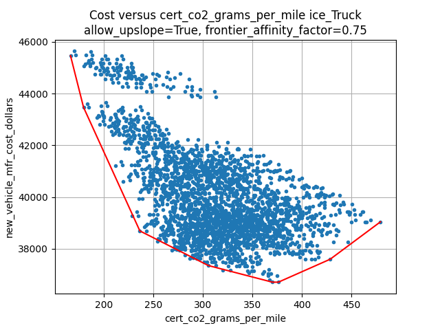
Fig. 7.1 Cost cloud and frontier,
o2.options.cost_curve_frontier_affinity_factor=0.75allow_upslope=TrueThese are the default settings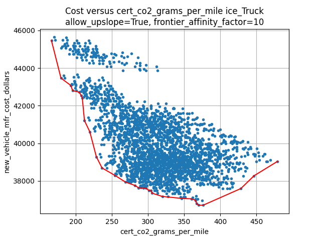
Fig. 7.2 Cost cloud and frontier,
o2.options.cost_curve_frontier_affinity_factor=10allow_upslope=TrueHigher affinity factor follows cloud points more closely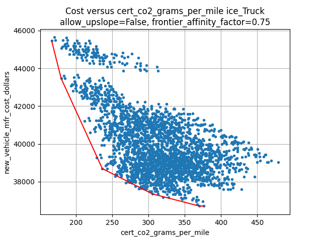
Fig. 7.3 Cost cloud and frontier,
o2.options.cost_curve_frontier_affinity_factor=0.75allow_upslope=FalseDefault affinity factor, no up-slope
-
calc_frontier_factor_down(cloud, prior_x, prior_y, x_key, y_key)¶ Calculate the frontier factor for an down-sloping cloud of points.
Parameters: - cloud (DataFrame) – a set of points to find the frontier of
- prior_x (float) – x-axis value of prior frontier point
- prior_y (float) – y-axis value of prior frontier point
- x_key (str) – name of the column holding x-axis data
- y_key (str) – name of the column holding y-axis data
Returns: Nothing, calculates
frontier_factorcolumn ofcloud.
-
calc_frontier_factor_up(cloud, prior_x, prior_y, x_key, y_key)¶ Calculate the frontier factor for an up-sloping cloud of points.
Parameters: - cloud (DataFrame) – a set of points to find the frontier of
- prior_x (float) – x-axis value of prior frontier point
- prior_y (float) – y-axis value of prior frontier point
- x_key (str) – name of the column holding x-axis data
- y_key (str) – name of the column holding y-axis data
Returns: Nothing, calculates
frontier_factorcolumn ofcloud.
-
calc_roadload_hp(A_LBSF, B_LBSF, C_LBSF, MPH)¶ Calculate roadload horsepower from ABC coefficients and vehicle speed (MPH)
Parameters: - A_LBSF (float) – “A” coefficient, lbs
- B_LBSF (float) – “B” coefficient, lbs/mph
- C_LBSF (float) – “C” coefficient, lbs/mph^2
- MPH (float(s)) – scalar float, numpy array or Series of vehicle speed(s), mph
Returns: Roadload horsepower at the given vehicle speed
-
cartesian_prod(left_df, right_df)¶ Calculate cartesian product of the dataframe rows.
Parameters: - left_df (DataFrame) – ‘left’ dataframe
- right_df (DataFrame) – ‘right’ dataframe
Returns: Cartesian product of the dataframe rows (the combination of every row in the left dataframe with every row in the right dataframe).
-
cull_cloud(cloud, prior_x, x_key)¶ Remove points from a dataframe where the given column (
x_key) is above a certain value (prior_x).Parameters: - cloud (dataframe) – the dataframe to cull
- prior_x (float) – the threshold value
- x_key (str) – cloud column name
Returns: cloudwith culled points removed
-
dataframe_to_numeric(df)¶ Convert dataframe columns to numeric (i.e. non-object dtypes) if possible.
Parameters: df (DataFrame) – the dataframe to convert to numeric Returns: df with numeric columns where possible
-
distribute_by_attribute(obj_list, value, weight_by, distribute_to)¶ Used to take a value and distribute it to source values by a weight factor. Used to assign composite attributes to source objects, e.g. composite vehicle sales to source vehicle sales, etc. The weight factor is normalized by the sum of the object weights. For example, if there were two objects, one with a 0.2 weight and one with a 0.1 weight, the first object would get 2/3 of the value and the second would get 1/3 of the value.
Parameters: - obj_list ([objs]) – list of objects to distribute to
- value (numeric) – the value to to distribute
- weight_by (str) – the name of the object attribute to use as a weight factor
- distribute_to (str) – the name of the object attribute to distribute to
Generate a partition of share values in the neighborhood of an initial set of share values.
See also
compliance_strategy.create_compliance_options()Parameters: - columns ([strs]) – list of values that represent shares in combo
- combos (Series, DataFrame) – typically a Series or Dataframe that contains the initial set of share values
- half_range_frac (float) – search “radius” [0..1], half the search range
- num_steps (int) – number of values to divide the search range into
- min_constraints (dict) – minimum partition constraints [0..1], by column name
- max_constraints (dict) – maximum partition constraints [0..1], by column name
- verbose (bool) – if
Truethen partition dataframe is printed to the console
Returns: DataFrame of partion values.
Example
>>>columns
['producer_share_frac_non_hauling.BEV', 'producer_share_frac_non_hauling.ICE']

>>>combos
      veh_non_hauling.BEV.car_co2e_gpmi  ...  slope
1510                          15.91862  ...      0
2135                          15.91862  ...      0
[2 rows x 79 columns]

>>>half_range_frac
0.33

>>>num_steps
5

>>>min_constraints
{'producer_share_frac_non_hauling.BEV': 0.001, 'producer_share_frac_non_hauling.ICE': 0}

>>>max_constraints
{'producer_share_frac_non_hauling.BEV': 1, 'producer_share_frac_non_hauling.ICE': 1}

Returns:
   producer_share_frac_non_hauling.BEV  producer_share_frac_non_hauling.ICE
0                               0.0010                               0.9990
1                               0.0835                               0.9165
2                               0.1660                               0.8340
3                               0.2485                               0.7515
4                               0.3310                               0.6690
5                               0.0010                               0.9990
Note
In the example above, there appear to be repeated rows, however the values are unique in floating-point terms, e.g. 0.00100000000000000002 versus 0.00100000000000000089
-
get_idxmin(cloud, min_frontier_factor, x_key)¶ Return the index of the minimum value of the
cloudfrontier_factor.Parameters: - cloud (DataFrame) – a set of points to find the frontier of
- min_frontier_factor (float) – the minimum value of the frontier_factor
- x_key (str) –
cloudcolumn name
Returns: The index of the minimum value of the
cloudfrontier_factor.
-
get_ip_address()¶ Attempt to get “local” IP address(es)
Example:
>>> socket.gethostbyname_ex(socket.gethostname())
('mac-mini.local', [], ['127.0.0.1', '192.168.1.20'])
Returns: list of local IP address(es)
-
linspace(min_val, max_val, num_values)¶ Create a list of num_values evenly spaced values between min and max. Based on
Matlablinspace command.Parameters: - min_val (numeric) – the minimum value
- max_val (numeric) – the maximum value
- num_values (int) – the total number of values to return
Returns: A list of evenly spaced values between min and max
-
partition(column_names, num_levels=5, min_constraints=None, max_constraints=None, verbose=False)¶ Generate a dataframe with columns from
column_names, whose rows sum to 1.0 across the columns, following the given constraintsParameters: - column_names – list of column names
- num_levels – number of values in the column with the lowest span (min value minus max value)
- min_constraints – a scalar value or dict of minimum value constraints with column names as keys
- max_constraints – a scalar value or dict of maximum value constraints with column names as keys
- verbose – if True then the resulting partition will be printed
Returns: A dataframe of the resulting partition
Example
p = partition_x(['BEV','ICE','PHEV'],
    min_constraints={'BEV':0.1},
    max_constraints={'BEV':0.2, 'PHEV':0.25},
    num_levels=5, verbose=True)
-
plot_frontier(cost_cloud, cost_curve_name, frontier_df, x_key, y_key)¶ Plot a cloud and its frontier. Saves plot to
o2.options.output_folder.Parameters: - cost_cloud (DataFrame) – set of points to plot
- cost_curve_name (str) – name of plot
- frontier_df (DataFrame) – set of points on the frontier
- x_key (str) – column name of x-value
- y_key (str) – columns name of y-value
Example
# from calc_cost_curve() in vehicles.py
plot_frontier(self.cost_cloud, '', cost_curve, 'cert_co2e_grams_per_mile', 'new_vehicle_mfr_cost_dollars')
-
print_dict(dict_in, num_tabs=0, to_string=False)¶ Attempt to printy-print a dictionary to the Python console.
Parameters: - dict_in (dict) – dictionary to print
- num_tabs (int) – optional argument, used to indent subsequent layers of the dictionary
- to_string (Bool) – if True then result will be returned as a printable string, instead of printed to the console
Returns: print_dict string if to_string==True
-
print_keys(dict_in, include=None, exclude=None, values=True)¶ Print some or all keys (and optionally values) in a dict-like object
Parameters: - dict_in (dict-like) – the object with keys to print
- include (str) – a substring that must be present, if provided
- exclude (str) – a substring that must not be present, if provided
- values (bool) – print values if
True
-
print_list(list_in)¶ Print the given list, one line per item
Parameters: list_in (list) – the list to print
-
sales_weight_average_dataframe(df)¶ - Numeric columns are sales-weighted-averaged except for ‘model_year’ and columns containing ‘sales’, which is the weighting factor. Non-numeric columns have unique values joined by ‘:’
Parameters: df (DataFrame) – the dataframe to sales-weight Returns: DataFrame with sales-weighted-average for numeric columns
-
send_text(dest, message, email, password)¶ SMS Gateways for each Carrier AT&T: [number]@txt.att.net Sprint: [number]@messaging.sprintpcs.com or [number]@pm.sprint.com T-Mobile: [number]@tmomail.net Verizon: [number]@vtext.com Boost Mobile: [number]@myboostmobile.com Cricket: [number]@sms.mycricket.com Metro PCS: [number]@mymetropcs.com Tracfone: [number]@mmst5.tracfone.com U.S. Cellular: [number]@email.uscc.net Virgin Mobile: [number]@vmobl.com
Parameters: - dest (str) – e.g. ‘8005552323@myboostmobile.com’
- message (str) – the message to send
- email (str) – the email address of the email server to use, e.g. ‘my_email@gmail.com’
- password (str) – the password for the email account, recommend setting up an app-specific password
-
series_to_numeric(ser)¶ Convert series entries to numeric (i.e. non-object dtypes) if possible.
Parameters: ser (Series) – the series to convert to numeric Returns: ser with numeric columns where possible
-
sum_dict(dict_in, include=None, exclude=None)¶ Add up all terms in a dict given the
includeandexcludeconstraints.Parameters: - dict_in (numeric dict_like) – the object with elements to sum
- include (str) – include term in sum if
includein dict key - exclude (str) – exclude term from some if
excludein dict key
Returns: Sum of terms in
dict_ingiven the include and exclude constraints.
-
unique(vector)¶ Return unique values in a list of values, in order of appearance.
Parameters: vector ([numeric]) – list of values Returns: List of unique values, in order of appearance
-
weighted_value(objects, weight_attribute, attribute, attribute_args=None)¶ Calculate a weighted value from values taken from a set of objects. The contribution of each object is normalized by the sum of the object weight attribute values.
Parameters: - objects ([objs]) – list of source objects
- weight_attribute (str) – the name of the object attribute to weight by (e.g. ‘sales’)
- attribute (str) – the name of the attribute to calculate the weighted value of, e.g. vehicle CO2e g/mi, etc
- attribute_args – arguments to the attribute, if the attribute is a method or function, e.g. calendar_year
Returns: The weighted value
7.3.1.1.8. omega_model.common.omega_globals module
OMEGA global variables.
Runtime options and database connection variables to be populated during initialization.
CODE
-
constraints= {}¶ dict of constraint dicts by market category
-
cumulative_battery_GWh= {'total': 0}¶ holds cumulative battery GWh production, by calendar year, from first pass
-
engine= None¶ connection to database engine
-
locked_price_modification_data= None¶ holds price locked modification data for the current compliance_id and calendar year
-
manufacturer_aggregation= False¶ true if manufacturer-level detail in vehicle aggregation
-
options= None¶ simulation options
-
pass_num= 0¶ multi-pass pass number
-
price_modification_data= None¶ holds price modification data for the current compliance_id and calendar year
producer shares mode when True
-
session= None¶ database session
round to the Nth digit when calculating share values in constraint dicts
7.3.1.1.9. omega_model.common.omega_log module
Functions to manage batch and session log files.
CODE
-
class
IterationLog(logfilename)¶ Bases:
common.omega_types.OMEGABaseHandles creation and writing of a dataframe to a .csv file, possibly multiple times via appending. Used to log producer-consumer iteration, but could be used to log any dataframe.
-
__init__(logfilename)¶ Create IterationLog object
Parameters: logfilename – name of file to create, ‘.csv’ extension added if not provided.
-
write(dataframe)¶ Write dataframe to a .csv file, file is created on first write, subsequent writes append.
Parameters: dataframe (DataFrame) – dataframe to write to file
-
-
class
OMEGABatchLog(o2_options, verbose=True)¶ Bases:
common.omega_types.OMEGABaseHandles logfile creation at the batch level.
-
__init__(o2_options, verbose=True)¶ Create OMEGABatchLog object
Parameters: - o2_options (OMEGABatchOptions) – provides the logfile name
- verbose (bool) – if True enables optional output to console as well as logfile
-
end_logfile(message)¶ End logfile with closing message, record elapsed time.
Parameters: message (str) – message string to write
-
logwrite(message, terminator='\n')¶ Write a message to a logfile (and console if verbose)
Parameters: - message (str) – message string to write
- terminator (str) – end of message terminator, default is newline (
\n)
-
-
end_logfile(message)¶ End logfile with closing message, record elapsed time.
Parameters: message (str) – message string to write
-
init_logfile()¶ Create a session logfile.
-
logwrite(message, echo_console=True, terminator='\n')¶ Write message to logfile.
Parameters: - message (str or [strs]) – message string or list of strings to write
- echo_console (bool) – write message to console if True
- terminator (str) – end of message terminator, default is newline (
\n)
7.3.1.1.10. omega_model.common.omega_plot module
Handy plotting functions for matplotlib plots.
CODE
-
figure(reuse_figure=False)¶ Create a figure window with a single plot axis.
Returns: 2-tuple of figure and axis objects, respectively.
-
fplothg(x, y, *args, reuse_figure=False, **kwargs)¶ Shortcut for figure, plot, hold on, grid on (based on Matlab plotting terminology) Creates a single axis plot, with grid.
Parameters: - x – x-values of data to plot
- y – y-values of data to plot
- *args – optional positional arguments to pyplot.plot()
- reuse_figure (bool) – re-use figure window if
True - **kwargs – optional keyword arguments to pyplot.plot()
Returns: 2-tuple of figure and axis objects, respectively.
-
fplotyyhg(x, y, ylinespec, y2, y2linespec)¶ Shortcut for figure, plotyy, hold on, grid on (based on Matlab plotting terminology). Creates a plot with a double y-axis and grid.
Parameters: - x – x-values of data to plot
- y – y-values of data to plot on first y-axis
- ylinespec (str) – line format string, e.g. ‘b.-’
- y2 – y-values of data to plot on second y-axis
- y2linespec (str) – line format string, e.g. ‘r.-’
Returns: 3-tuple of figure and two axis objects, respectively.
-
label_xy(ax, x_label_str, y_label_str)¶ Label x-axis and y-axis.
Parameters: - ax (matplotlib.axes._subplots.AxesSubplot) – the axis (plot) to label
- x_label_str (str) – x-axis label
- y_label_str (str) – y-axis label
-
label_xyt(ax, x_label_str, y_label_str, title_str)¶ Label x-axis, y-axis and set axis title.
Parameters: - ax (matplotlib.axes._subplots.AxesSubplot) – the axis(plot) to label
- x_label_str (str) – x-axis label
- y_label_str (str) – y-axis label
- title_str (str) – axis title
Returns:
-
lineat(ax, y, *args, **kwargs)¶ Draw a horizontal line at a y-value.
Parameters: - ax (matplotlib.axes._subplots.AxesSubplot) – the axis (plot) to draw on
- y (numeric) – the vertical index of the line
- *args – optional positional arguments to pyplot.plot()
- **kwargs – optional keyword arguments to pyplot.plot()
-
vlineat(ax, x, *args, **kwargs)¶ Draw a vertical line at an x-value.
Parameters: - ax (matplotlib.axes._subplots.AxesSubplot) – the axis to draw on
- x (numeric) – the horizontal index of the line
- *args – optional positional arguments to pyplot.plot()
- **kwargs – optional keyword arguments to pyplot.plot()
7.3.1.1.11. omega_model.common.omega_trees module
Routines and data structures for tree-based algorithms and functions.
CODE
-
class
WeightedNode(weight)¶ Bases:
common.omega_types.OMEGABaseImplements nodes in a tree where nodes have weights and values. Used for drive cycle weighting, but could also be used for weighting in general, if needed.
WeightedNodesare stored as node data in aWeightedTree.tree(see below), which is atreelib.Tree.-
__init__(weight)¶ Create WeightedNode
Parameters: weight (numeric) – node weight
-
identifier¶ Generate a node ID string.
Returns: Node ID string.
-
weighted_value¶ Calculate node weighted value.
Returns: Node weight times node value if weight is not None, else returns 0.
-
-
class
WeightedTree(tree_df, verbose=False)¶ Bases:
common.omega_types.OMEGABaseImplements a tree data structure of
WeightedNodesand methods of querying node values.-
__init__(tree_df, verbose=False)¶ Create WeightedTree from a dataframe containing node connections as column headers and weights as row values.
Parameters: - tree_df (DataFrame) – a dataframe with column headers such as
'A->B', 'A->C', 'B->D'etc. - verbose (bool) – prints the tree to the console if True
Note
The first element of the first column containing an arrow (
->) is taken as the root node. Parent nodes must be referenced before child nodes, otherwise there is no particular pre-defined order. In the above example, B is a child of A before D can be a child of B.- tree_df (DataFrame) – a dataframe with column headers such as
-
static
calc_node_weighted_value(tree, node_id)¶ Calculate node weighted value. If the node has no children then the weighted value is the node’s weighted value, see
WeightedNodeabove. If the node has children then the weighted value is the sum of the weighted values of the children, recursively if necessary.Parameters: - tree (treelib.Tree) – the tree to query
- node_id (str) – the id of the node to query
Returns: Node weighted value
-
calc_value(values_dict, node_id=None, weighted=False)¶ Assign values to tree leaves then calculate the value or weighted value at the given
node_idor at the root if nonode_idis provided. Previously calculated values are cleared first.Parameters: - values_dict (dict-like) – values to assign to leaves
- node_id (str) – node id to calculate weighted value of, or tree root if not provided
- weighted (bool) – if True then return weighted value, else return node value
Returns: Node (or tree) value (or weighted value)
-
leaves()¶ Get list of tree leaves.
Returns: List of tree nodes (type treelib.node.Node) that have no children.
-
show()¶ Print the tree to the console.
-
validate_weights()¶ Validated node weights. The sum of a parent node’s child node weights must equal 1.0. Nodes with a weight of
Noneare ignored during summation.Returns: List of node weight errors, or empty list on success.
-
7.3.1.1.12. omega_model.common.omega_types module
Custom general datatypes for use in OMEGA.
CODE
-
class
OMEGABase¶ Bases:
objectDefines a base class with common behaviors for all OMEGA objects.
Example of representation strings and printing via
__repr__and__str__methods:class ExampleOMEGAClass(OMEGABase): def __init__(self): self.first_attribute = 0 self.second_attribute = 1 >>>example_object = ExampleOMEGAClass() >>>example_object <OMEGA2 ExampleOMEGAClass object at 0x7f91d03975e0> >>>print(example_object) <OMEGA2 ExampleOMEGAClass object at 0x7f91d03975e0> first_attribute = 0 second_attribute = 1
-
classmethod
get_class_attributes(attribute_list)¶ Get a list of class attributes.
Parameters: - cls (class) – the class to get attributes from
- attribute_list ([strs]) – a list of attribute names
Returns: A list containing the values of the requested attributes
-
__repr__()¶ Generate a representation string for the object.
Returns: A string representation of the object.
-
__str__()¶ Generate a string of object attributes, so objects have a default print behavior.
Returns: A string with a listing of object attributes and values.
-
get_object_attributes(attribute_list)¶ Get a list of object attributes.
Parameters: - self (object) – the object to get attributes from
- attribute_list ([strs]) – a list of attribute names
Returns: A list containing the values of the requested attributes
-
classmethod
-
class
OMEGAEnum(enum_list)¶ Bases:
omega_model.common.omega_types.OMEGABaseSimple enumerated value class, which acts like a list of strings, has named attributes which contain the attribute name as a string, also acts like a dictionary.
Example
# define an OMEGAEnum
reg_classes = OMEGAEnum(['car', 'truck'])

# named attribute behavior
>>>reg_classes.car
'car'

# dict-like behavior
>>>reg_classes['car']
'car'

>>>reg_classes.keys()
dict_keys(['car', 'truck'])

>>>reg_classes.values()
dict_values(['car', 'truck'])

>>>reg_classes.items()
dict_items([('car', 'car'), ('truck', 'truck')])

# list-like behavior
>>>[rc for rc in reg_classes]
['car', 'truck']
-
__init__(enum_list)¶ Create OMEGAEnum object from list of values.
Parameters: enum_list (list) – list of enumeration values
-
items()¶ Implement items() function, like a dict.
Returns: A list of key-value pairs (2-tuples)
-
keys()¶ Implement keys() function, like a dict.
Returns: A list of keys
-
values()¶ Implement values() function, like a dict.
Returns: A list of values
-
-
make_valid_python_identifier(s)¶ Creates a valid python identifier from a source string (by removing invalid characters).
Parameters: s (str) – the source string to make a valid identifier from Returns: A valid python identifier based on the source string
7.3.1.2. omega_model.consumer package
The consumer package defines market classes, their associated properties, and routines to determine consumer desired market shares as a function of market class, relative costs, etc. The consumer module also handles vehicle re-registration.
CODE
7.3.1.2.1. Submodules
7.3.1.2.2. omega_model.consumer.annual_vmt_fixed_by_age module
Routines to load and provide access to annual vehicle miles travelled (VMT) by market class and age.
The data represents a fixed VMT schedule by age.
INPUT FILE FORMAT
The file format consists of a one-row template header followed by a one-row data header and subsequent data rows. The template header uses a dynamic format.
The data represents the re-registered proportion of vehicles by calendar year, age and market class.
- File Type
- comma-separated values (CSV)
- Template Header
input_template_name: [module_name]input_template_version: [template_version]- Sample Header
input_template_name: consumer.annual_vmt_fixed_by_age input_template_version: 0.2 - Sample Data Columns
start_year age market_class_id annual_vmt 2019 0 non_hauling.BEV 14699.55515 2019 1 non_hauling.BEV 14251.70373 2019 2 non_hauling.BEV 14025.35397 2019 0 hauling.ICE 15973.88982 2019 1 hauling.ICE 15404.1216 2019 2 hauling.ICE 14840.93011
| start_year: | Start year of annual VMT data, values apply until the next available start year |
|---|---|
| age: | Vehicle age, in years |
| market_class_id: | |
| Vehicle market class ID, e.g. ‘hauling.ICE’ | |
| annual_vmt: | Vehicle miles travelled per year at the given age for the given market class ID |
CODE
-
class
OnroadVMT¶ Bases:
common.omega_types.OMEGABase,consumer.consumer_base_classes.AnnualVMTBaseLoads and provides access to annual Vehicle Miles Travelled by calendar year, market class, and age.
-
cumulative_vmt= {}
-
static
get_cumulative_vmt(market_class_id, age)¶ Get the cumulative VMT for the given market class and age
Parameters: - market_class_id (str) – market class id, e.g. ‘hauling.ICE’
- age (int) – vehicle age in years
Returns: The cumulative VMT for the given market class and age
-
static
get_vmt(calendar_year, market_class_id, age)¶ Get vehicle miles travelled by calendar year, market class and age.
Parameters: - calendar_year (int) – calendar year of the VMT data
- market_class_id (str) – market class id, e.g. ‘hauling.ICE’
- age (int) – vehicle age in years
Returns: (float) Annual vehicle miles travelled.
-
static
init_from_file(filename, verbose=False)¶ Initialize class data from input file.
Parameters: - filename (str) – name of input file
- verbose (bool) – enable additional console and logfile output if True
Returns: List of template/input errors, else empty list on success
-
7.3.1.2.3. omega_model.consumer.consumer_base_classes module
A set of base classes used to define the program interface(s) and to serve as templates for user-defined classes
Ordinarily these classes might be implemented as Python abstract classes but abstract classes cause issues when combined with SQLAlchemy base classes, so the implementation here is a workaround - if a child class fails to implement one of the required methods, the class will throw a runtime Exception or return an error message.
-
class
AnnualVMTBase¶ Bases:
objectLoads and provides access to annual Vehicle Miles Travelled by calendar year, market class, and age.
-
static
get_vmt(calendar_year, market_class_id, age)¶ Get vehicle miles travelled by calendar year, market class and age.
Parameters: - calendar_year (int) – calendar year of the VMT data
- market_class_id (str) – market class id, e.g. ‘hauling.ICE’
- age (int) – vehicle age in years
Returns: (float) Annual vehicle miles travelled.
-
static
init_from_file(filename, verbose=False)¶ Initialize class data from input file.
Parameters: - filename (str) – name of input file
- verbose (bool) – enable additional console and logfile output if True
Returns: List of template/input errors, else empty list on success
-
static
-
class
MarketClassBase¶ Bases:
objectLoads market class definition data and provides market-class-related functionality.
-
static
get_market_class_dict()¶ Get a copy of the market class dict with an empty list for each market class.
Returns: A copy of the market class dict.
-
static
get_market_class_tree(by_reg_class=False)¶ Get a copy of a hierarchical market class dict with empty lists for each market class or by regulatory class within the market class.
Parameters: by_reg_class (bool) – if True then return a tree by reg class within market class. Returns: A copy of the appropriate hierarchical market class dict.
-
static
get_non_responsive_market_category(market_class_id)¶ Returns the non-responsive market category of the given market class ID
Parameters: market_class_id (str) – market class ID, e.g. ‘hauling.ICE’ Returns: The non-responsive market category of the given market class ID
-
static
get_vehicle_market_class(vehicle)¶ Get vehicle market class ID based on vehicle characteristics
Parameters: vehicle (VehicleFinal) – the vehicle to determine the market class of Returns: The vehicle’s market class ID based on vehicle characteristics.
-
static
init_from_file(filename, verbose=False)¶ Initialize class data from input file.
Parameters: - filename (str) – name of input file
- verbose (bool) – enable additional console and logfile output if True
Returns: List of template/input errors, else empty list on success
-
linked_market_classes= {}
-
market_categories= []
-
market_classes= ()¶ tuple of market classes
-
non_responsive_market_categories= []
-
static
parse_market_classes(market_class_list, market_class_dict=None, by_reg_class=False)¶ Returns a nested dictionary of market classes from a dot-formatted list of market class names.
Parameters: - market_class_list ([strs]) – list of dot-separted market class names e.g. [‘hauling.BEV’, ‘hauling.ICE’] etc
- market_class_dict (dict, dict of dicts) – recursive input and also the output data structure
- by_reg_class (bool) – if true then leaves are lists in reg class dicts, otherwise leaves are lists by market segment
Returns: Market class tree represented as a dict or dict of dicts, with an empty list at each leaf. e.g.
{'non_hauling': {'BEV': [], 'ICE': []}, 'hauling': {'BEV': [], 'ICE': []}}
-
static
populate_market_classes(market_class_dict, market_class_id, obj)¶ Populate the leaves of a market class tree implemented as a dict (or dict of dicts) where the keys represent market categories and the leaves are lists of objects grouped by market class.
Parameters: - market_class_dict (dict) – dict of dicts of market classes
- market_class_id (str) – dot separated market class name e.g. ‘hauling.BEV’, possibly with reg class suffix e.g. ‘non_hauling.ICE.car’ depending on the market_class_dict
- obj (object) – object to place in a list in the appropriate leaf, as in a CompositeVehicle
Returns: Nothing, modifies
market_class_dictdata
-
responsive_market_categories= []
-
static
validate_market_class_id(market_class_id)¶ Validate market class ID
Parameters: market_class_id (str) – market class ID, e.g. ‘hauling.ICE’ Returns: Error message in a list if market_class_id is not valid
-
static
-
class
ReregistrationBase¶ Bases:
objectLoad and provide access to vehicle re-registration data by model year, market class ID and age.
-
static
get_reregistered_proportion(model_year, market_class_id, age)¶ Get vehicle re-registered proportion [0..1] by market class and age.
Parameters: - model_year (int) – the model year of the re-registration data
- market_class_id (str) – market class id, e.g. ‘hauling.ICE’
- age (int) – vehicle age in years
Returns: Re-registered proportion [0..1]
-
static
init_from_file(filename, verbose=False)¶ Initialize class data from input file.
Parameters: - filename (str) – name of input file
- verbose (bool) – enable additional console and logfile output if True
Returns: List of template/input errors, else empty list on success
-
static
Bases:
objectClass to calculate absolute market shares by market class
- Calculate base year data (if necessary) such as sales-weighted curbweight, etc, if needed for reference in future years
Parameters: base_year_vehicles_df (DataFrame) – base year vehicle data
Determine consumer desired market shares for the given vehicles, their costs, etc. Relative shares are first calculated within non-responsive market categories then converted to absolute shares.
Parameters: - calendar_year (int) – calendar year to calculate market shares in
- compliance_id (str) – manufacturer name, or ‘consolidated_OEM’
- producer_decision (Series) – selected producer compliance option
- market_class_data (DataFrame) – DataFrame with ‘average_fuel_price_MC’, ‘average_modified_cross_subsidized_price_MC’, ‘average_co2e_gpmi_MC’, ‘average_kwh_pmi_MC’ columns, where MC = market class ID
- mc_parent (str) – e.g. ‘’ for the total market, ‘hauling’ or ‘non_hauling’, etc
- mc_pair ([strs]) – e.g. ‘[‘hauling’, ‘non_hauling’] or [‘hauling.ICE’, ‘hauling.BEV’], etc
Returns: A copy of
market_class_datawith demanded ICE/BEV share columns by market class, e.g. ‘consumer_share_frac_MC’, ‘consumer_abs_share_frac_MC’, and ‘consumer_generalized_cost_dollars_MC’ where MC = market class ID
Initialize class data from input file.
Parameters: - filename (str) – name of input file
- verbose (bool) – enable additional console and logfile output if True
Returns: List of template/input errors, else empty list on success
- Save calibration data (if necessary) that aligns reference session market shares with context
Parameters: filename (str) – name of the calibration file
- Store producer decision and response (if necessary) for reference in future years
Parameters: producer_decision_and_response (Series) – producer decision and consumer response
7.3.1.2.4. omega_model.consumer.market_classes_body_style module
Routines to implement market-class related functionality.
INPUT FILE FORMAT
The file format consists of a one-row template header followed by a one-row data header and subsequent data rows. The template header uses a dynamic format.
The data represents characteristics of the Consumer Module’s market classes.
- File Type
- comma-separated values (CSV)
- Template Header
input_template_name: [module_name]input_template_version: [template_version]- Sample Header
input_template_name: consumer.market_classes_body_style input_template_version: 0.1 - Sample Data Columns
market_class_id fueling_class ownership_class sedan_wagon.BEV BEV private cuv_suv_van.ICE ICE private
Data Column Name and Description
| market_class_id: | |
|---|---|
| Vehicle market class ID, e.g. ‘sedan_wagon.ICE’ | |
| fueling_class: | Market class fueling class, e.g. ‘BEV’, ‘ICE’ |
| ownership_class: | |
| Market class ownership class, e.g. ‘private’, ‘shared’ (For future development) | |
CODE
-
class
MarketClass¶ Bases:
common.omega_types.OMEGABase,consumer.consumer_base_classes.MarketClassBaseLoads market class definition data and provides market-class-related functionality.
-
static
get_non_responsive_market_category(market_class_id)¶ Returns the non-responsive market category of the given market class ID
Parameters: market_class_id (str) – market class ID, e.g. ‘hauling.ICE’ Returns: The non-responsive market category of the given market class ID
-
static
get_vehicle_market_class(vehicle)¶ Get vehicle market class ID based on vehicle characteristics
Parameters: vehicle (VehicleFinal) – the vehicle to determine the market class of Returns: The vehicle’s market class ID based on vehicle characteristics.
-
static
init_from_file(filename, verbose=False)¶ Initialize class data from input file.
Parameters: - filename (str) – name of input file
- verbose (bool) – enable additional console and logfile output if True
Returns: List of template/input errors, else empty list on success
-
market_categories= ['ICE', 'BEV', 'sedan_wagon', 'cuv_suv_van', 'pickup']¶ overall market categories
-
non_responsive_market_categories= ['sedan_wagon', 'cuv_suv_van', 'pickup']¶ market categories that do not have consumer response
-
responsive_market_categories= ['ICE', 'BEV']¶ market categories that have consumer response (i.e. price -> sales)
-
static
validate_market_class_id(market_class_id)¶ Validate market class ID
Parameters: market_class_id (str) – market class ID, e.g. ‘hauling.ICE’ Returns: Error message in a list if market_class_id is not valid
-
static
7.3.1.2.5. omega_model.consumer.market_classes_body_style_zevregion module
Routines to implement market-class related functionality.
INPUT FILE FORMAT
The file format consists of a one-row template header followed by a one-row data header and subsequent data rows. The template header uses a dynamic format.
The data represents characteristics of the Consumer Module’s market classes.
- File Type
- comma-separated values (CSV)
- Template Header
input_template_name: [module_name]input_template_version: [template_version]- Sample Header
input_template_name: consumer.market_classes_body_style_zevregion input_template_version: 0.1 - Sample Data Columns
market_class_id fueling_class ownership_class sedan_wagon_r1nonzev.BEV BEV private cuv_suv_van_r2zev.ICE ICE private
Data Column Name and Description
| market_class_id: | |
|---|---|
| Vehicle market class ID, e.g. ‘sedan_wagon_r1nonzev.ICE’ | |
| fueling_class: | Market class fueling class, e.g. ‘BEV’, ‘ICE’ |
| ownership_class: | |
| Market class ownership class, e.g. ‘private’, ‘shared’ (For future development) | |
CODE
-
class
MarketClass¶ Bases:
common.omega_types.OMEGABase,consumer.consumer_base_classes.MarketClassBaseLoads market class definition data and provides market-class-related functionality.
-
static
get_non_responsive_market_category(market_class_id)¶ Returns the non-responsive market category of the given market class ID
Parameters: market_class_id (str) – market class ID, e.g. ‘hauling.ICE’ Returns: The non-responsive market category of the given market class ID
-
static
get_vehicle_market_class(vehicle)¶ Get vehicle market class ID based on vehicle characteristics
Parameters: vehicle (VehicleFinal) – the vehicle to determine the market class of Returns: The vehicle’s market class ID based on vehicle characteristics.
-
static
init_from_file(filename, verbose=False)¶ Initialize class data from input file.
Parameters: - filename (str) – name of input file
- verbose (bool) – enable additional console and logfile output if True
Returns: List of template/input errors, else empty list on success
-
linked_market_classes= {'cuv_suv_van_r2zev.ICE': 'cuv_suv_van_r1nonzev.ICE', 'pickup_r2zev.ICE': 'pickup_r1nonzev.ICE', 'sedan_wagon_r2zev.ICE': 'sedan_wagon_r1nonzev.ICE'}
-
market_categories= ['ICE', 'BEV', 'sedan_wagon_r1nonzev', 'cuv_suv_van_r1nonzev', 'pickup_r1nonzev', 'sedan_wagon_r2zev', 'cuv_suv_van_r2zev', 'pickup_r2zev']¶ overall market categories
-
non_responsive_market_categories= ['sedan_wagon_r1nonzev', 'cuv_suv_van_r1nonzev', 'pickup_r1nonzev', 'sedan_wagon_r2zev', 'cuv_suv_van_r2zev', 'pickup_r2zev']¶ market categories that do not have consumer response
-
responsive_market_categories= ['ICE', 'BEV']¶ market categories that have consumer response (i.e. price -> sales)
-
static
validate_market_class_id(market_class_id)¶ Validate market class ID
Parameters: market_class_id (str) – market class ID, e.g. ‘hauling.ICE’ Returns: Error message in a list if market_class_id is not valid
-
static
7.3.1.2.6. omega_model.consumer.market_classes_legacy_reg_class module
Routines to implement market-class related functionality.
INPUT FILE FORMAT
The file format consists of a one-row template header followed by a one-row data header and subsequent data rows. The template header uses a dynamic format.
The data represents characteristics of the Consumer Module’s market classes.
- File Type
- comma-separated values (CSV)
- Template Header
input_template_name: [module_name]input_template_version: [template_version]- Sample Header
input_template_name: consumer.market_classes_legacy_reg_class input_template_version: 0.32 - Sample Data Columns
market_class_id fueling_class ownership_class non_hauling.BEV BEV private hauling.ICE ICE private
Data Column Name and Description
| market_class_id: | |
|---|---|
| Vehicle market class ID, e.g. ‘hauling.ICE’ | |
| fueling_class: | Market class fueling class, e.g. ‘BEV’, ‘ICE’ |
| ownership_class: | |
| Market class ownership class, e.g. ‘private’, ‘shared’ (For future development) | |
CODE
-
class
MarketClass¶ Bases:
common.omega_types.OMEGABase,consumer.consumer_base_classes.MarketClassBaseLoads market class definition data and provides market-class-related functionality.
-
static
get_non_responsive_market_category(market_class_id)¶ Returns the non-responsive market category of the given market class ID
Parameters: market_class_id (str) – market class ID, e.g. ‘hauling.ICE’ Returns: The non-responsive market category of the given market class ID
-
static
get_vehicle_market_class(vehicle)¶ Get vehicle market class ID based on vehicle characteristics
Parameters: vehicle (VehicleFinal) – the vehicle to determine the market class of Returns: The vehicle’s market class ID based on vehicle characteristics.
-
static
init_from_file(filename, verbose=False)¶ Initialize class data from input file.
Parameters: - filename (str) – name of input file
- verbose (bool) – enable additional console and logfile output if True
Returns: List of template/input errors, else empty list on success
-
market_categories= ['ICE', 'BEV', 'hauling', 'non_hauling']¶ overall market categories
-
non_responsive_market_categories= ['hauling', 'non_hauling']¶ market categories that do not have consumer response
-
responsive_market_categories= ['ICE', 'BEV']¶ market categories that have consumer response (i.e. price -> sales)
-
static
validate_market_class_id(market_class_id)¶ Validate market class ID
Parameters: market_class_id (str) – market class ID, e.g. ‘hauling.ICE’ Returns: Error message in a list if market_class_id is not valid
-
static
7.3.1.2.7. omega_model.consumer.market_classes_unibody module
Routines to implement market-class related functionality.
INPUT FILE FORMAT
The file format consists of a one-row template header followed by a one-row data header and subsequent data rows. The template header uses a dynamic format.
The data represents characteristics of the Consumer Module’s market classes.
- File Type
- comma-separated values (CSV)
- Template Header
input_template_name: [module_name]input_template_version: [template_version]- Sample Header
input_template_name: consumer.market_classes_unibody input_template_version: 0.32 - Sample Data Columns
market_class_id fueling_class ownership_class non_hauling.BEV BEV private hauling.ICE ICE private
Data Column Name and Description
| market_class_id: | |
|---|---|
| Vehicle market class ID, e.g. ‘hauling.ICE’ | |
| fueling_class: | Market class fueling class, e.g. ‘BEV’, ‘ICE’ |
| ownership_class: | |
| Market class ownership class, e.g. ‘private’, ‘shared’ (For future development) | |
CODE
-
class
MarketClass¶ Bases:
common.omega_types.OMEGABase,consumer.consumer_base_classes.MarketClassBaseLoads market class definition data and provides market-class-related functionality.
-
static
get_non_responsive_market_category(market_class_id)¶ Returns the non-responsive market category of the given market class ID
Parameters: market_class_id (str) – market class ID, e.g. ‘hauling.ICE’ Returns: The non-responsive market category of the given market class ID
-
static
get_vehicle_market_class(vehicle)¶ Get vehicle market class ID based on vehicle characteristics
Parameters: vehicle (VehicleFinal) – the vehicle to determine the market class of Returns: The vehicle’s market class ID based on vehicle characteristics.
-
static
init_from_file(filename, verbose=False)¶ Initialize class data from input file.
Parameters: - filename (str) – name of input file
- verbose (bool) – enable additional console and logfile output if True
Returns: List of template/input errors, else empty list on success
-
market_categories= ['ICE', 'BEV', 'hauling', 'non_hauling']¶ overall market categories
-
non_responsive_market_categories= ['hauling', 'non_hauling']¶ market categories that do not have consumer response
-
responsive_market_categories= ['ICE', 'BEV']¶ market categories that have consumer response (i.e. price -> sales)
-
static
validate_market_class_id(market_class_id)¶ Validate market class ID
Parameters: market_class_id (str) – market class ID, e.g. ‘hauling.ICE’ Returns: Error message in a list if market_class_id is not valid
-
static
7.3.1.2.8. omega_model.consumer.reregistration_fixed_by_age module
Vehicle re-registration, fixed by age.
INPUT FILE FORMAT
The file format consists of a one-row template header followed by a one-row data header and subsequent data rows. The template header uses a dynamic format.
The data represents the re-registered proportion of vehicles by model year, age and market class.
- File Type
- comma-separated values (CSV)
- Template Header
input_template_name: [module_name]input_template_version: [template_version]- Sample Header
input_template_name: consumer.reregistration_fixed_by_age input_template_version: 0.2 - Sample Data Columns
start_model_year age market_class_id reregistered_proportion 1970 0 non_hauling.BEV 1 1970 1 non_hauling.BEV 0.987841531 1970 2 non_hauling.BEV 0.976587217 1970 0 hauling.ICE 1 1970 1 hauling.ICE 0.977597055 1970 2 hauling.ICE 0.962974697
Data Column Name and Description
| start_model_year: | |
|---|---|
| The start vehicle model year of the re-registration data, values apply until next available start year | |
| age: | Vehicle age, in years |
| market_class_id: | |
| Vehicle market class ID, e.g. ‘hauling.ICE’ | |
| reregistered_proportion: | |
| The fraction of vehicles re-registered, [0..1] | |
CODE
-
class
Reregistration¶ Bases:
common.omega_types.OMEGABase,consumer.consumer_base_classes.ReregistrationBaseLoad and provide access to vehicle re-registration data by model year, market class ID and age.
-
static
get_reregistered_proportion(model_year, market_class_id, age)¶ Get vehicle re-registered proportion [0..1] by market class and age.
Parameters: - model_year (int) – the model year of the re-registration data
- market_class_id (str) – market class id, e.g. ‘hauling.ICE’
- age (int) – vehicle age in years
Returns: Re-registered proportion [0..1]
-
static
init_from_file(filename, verbose=False)¶ Initialize class data from input file.
Parameters: - filename (str) – name of input file
- verbose (bool) – enable additional console and logfile output if True
Returns: List of template/input errors, else empty list on success
-
static
7.3.1.2.13. omega_model.consumer.sales_volume module
Routines to retrieve overall sales from the context and total consumer sales response as a function of total sales-weighted generalized cost.
CODE
-
context_new_vehicle_sales(calendar_year)¶ Get new vehicle sales from the context.
Parameters: calendar_year (int) – the year to get sales for Returns: dict of vehicle sales by non-responsive market category, and total
-
init_sales_volume()¶ Initialize the module by clearing the cache.
-
log_new_vehicle_generalized_cost(calendar_year, compliance_id, P)¶ Parameters: - calendar_year (int) – the calendar year to calculate sales in
- compliance_id (str) – manufacturer name, or ‘consolidated_OEM’
- P ($, [$]) – a single price representing the final production decision average new vehicle generalized cost
-
new_vehicle_sales_response(calendar_year, compliance_id, P)¶ Calculate new vehicle sales fraction relative to a reference sales volume and average new vehicle generalized cost. Updates generalized cost table associated with the reference session so those costs can become the reference costs for subsequent sessions.
Parameters: - calendar_year (int) – the calendar year to calculate sales in
- compliance_id (str) – manufacturer name, or ‘consolidated_OEM’
- P ($, [$]) – a single price or a list/vector of prices
Returns: Relative new vehicle sales volume at each price, e.g.
0.97,1.03, etc
7.3.1.2.14. omega_model.consumer.stock module
Routines to implement vehicle re-registration on an annual basis as a function of vehicle attributes.
CODE
-
get_vehicle_info(vehicle_id)¶ Gets vehicle info for the given database vehicle ID
Parameters: vehicle_id (int) – the database vehicle ID (e.g. 1,2,3…) Returns: Vehicle market_class_id, model_year, initial_registered_count
-
update_stock(calendar_year, compliance_id=None)¶ Re-register vehicles by calendar year, as a function of vehicle attributes (e.g. age, market class…) Also calculates vehicle miles travelled for each vehilce by market class and age.
Parameters: - compliance_id (str) – optional argument, manufacturer name, or ‘consolidated_OEM’
- calendar_year (int) – calendar year to re-register vehicles in
Returns: Nothing, updates VehicleAnnualData entries (
age,registered_count,annual_vmt,vmt).
7.3.1.3. omega_model.context package
OMEGA analysis context subpackage
CODE
7.3.1.3.1. Submodules
7.3.1.3.2. omega_model.context.body_styles module
Routines to load, validate, and provide access to body style definition data
Body styles defined by a name and a brief description.
INPUT FILE FORMAT
The file format consists of a one-row template header followed by a one-row data header and subsequent data rows.
The data represents body style names and a brief description.
- File Type
- comma-separated values (CSV)
- Sample Header
input_template_name: body_styles input_template_version: 0.1 - Sample Data Columns
body_style_id description sedan Non-pickup / non-crossover / non-sport-utility vehicle pickup Pickup truck / body-on-frame vehicle cuv_suv Crossover / sport-utility vehicle
Data Column Name and Description
| body_style_id: | Name of the body style |
|---|---|
| description: | A brief description of the body style |
CODE
-
class
BodyStyles¶ Bases:
common.omega_types.OMEGABaseLoad and provides routines to access drive cycle descriptive data
-
body_styles= []¶ list of available body styles
-
static
init_from_file(filename, verbose=False)¶ Initialize class data from input file.
Parameters: - filename (str) – name of input file
- verbose (bool) – enable additional console and logfile output if True
Returns: List of template/input errors, else empty list on success
-
7.3.1.3.3. omega_model.context.context_base_classes module
Context base classes.
Currently just CostCloudBase.
-
class
CostCloudBase¶ Bases:
objectLoads and provides access to simulated vehicle data, provides methods to calculate and plot frontiers.
-
static
get_cloud(vehicle)¶ Retrieve cost cloud for the given vehicle.
Parameters: () (vehicle) – the vehicle to get the cloud for Returns: Copy of the requested cost cload data.
-
static
init_cost_clouds_from_files(ice_filename, bev_filename, phev_filename, verbose=False)¶ Initialize class data from input file.
Parameters: - ice_filename (str) – name of ICE/HEV vehicle simulation data input file
- bev_filename (str) – name of BEV vehicle simulation data input file
- phev_filename (str) – name of PHEV vehicle simulation data input file
- verbose (bool) – enable additional console and logfile output if True
Returns: List of template/input errors, else empty list on success
-
static
7.3.1.3.4. omega_model.context.fuel_prices module
Routines to load and access fuel prices from the analysis context
Context fuel price data includes retail and pre-tax costs in dollars per unit (e.g. $/gallon, $/kWh)
INPUT FILE FORMAT
The file format consists of a one-row template header followed by a one-row data header and subsequent data rows.
The data represents fuel prices by context case, fuel type, and calendar year.
- File Type
- comma-separated values (CSV)
- Sample Header
input_template_name: context_fuel_prices input_template_version: 0.2 - Sample Data Columns
context_id dollar_basis case_id fuel_id calendar_year retail_dollars_per_unit pretax_dollars_per_unit AEO2020 2019 Reference case pump gasoline 2019 2.665601 2.10838 AEO2020 2019 Reference case US electricity 2019 0.12559407 0.10391058 - Data Column Name and Description
context_id: The name of the context source, e.g. ‘AEO2020’, ‘AEO2021’, etc dollar_basis: The dollar basis of the fuel prices in the given AEO version. Note that this dollar basis is converted in-code to ‘analysis_dollar_basis’ using the implicit_price_deflators input file. case_id: The name of the case within the context, e.g. ‘Reference Case’, ‘High oil price’, etc fuel_id: The name of the vehicle in-use fuel, must be in the table loaded by class fuels.Fueland consistent with the base year vehicles file (columnin_use_fuel_id) loaded byclass vehicles.VehicleFinalcalendar_year: The calendar year of the fuel costs retail_dollars_per_unit: Retail dollars per unit pretax_dollars_per_unit: Pre-tax dollars per unit
CODE
-
class
FuelPrice¶ Bases:
common.omega_types.OMEGABaseLoads and provides access to fuel prices from the analysis context
-
static
get_fuel_prices(calendar_year, price_types, fuel_id)¶ - Get fuel price data for fuel_id in calendar_year
Parameters: - calendar_year (numeric) – calendar year to get price in
- price_types (str, [str1, str2...]) – ContextFuelPrices attributes to get
- fuel_id (str) – fuel ID
Returns: Fuel price or tuple of fuel prices if multiple attributes were requested
Example
pretax_pump_gas_price_dollars_2030 =
ContextFuelPrices.get_fuel_prices(2030, 'pretax_dollars_per_unit', 'pump gasoline')

pump_gas_attributes_2030 =
ContextFuelPrices.get_fuel_prices(2030, ['retail_dollars_per_unit', 'pretax_dollars_per_unit'], 'pump gasoline')
-
static
init_from_file(filename, verbose=False)¶ Initialize class data from input file.
Parameters: - filename (str) – name of input file
- verbose (bool) – enable additional console and logfile output if True
Returns: List of template/input errors, else empty list on success
-
static
7.3.1.3.5. omega_model.context.glider_cost module
Routines to calculate glider cost.
INPUT FILE FORMAT
The file format consists of a one-row template header followed by a one-row data header and subsequent data rows. The template header uses a dynamic format.
- File Type
- comma-separated values (CSV)
- Sample Header
input_template_name: glider_cost input_template_version: 0.11 notes: 20220719 structure costs for aluminum BIW aligned with FEV Venza and Silverado teardowns - Sample Data Columns
body_style item material value dollar_basis sedan unibody_structure steel (1.5 * structure_mass_lbs + 1500) * markup 2020 sedan unibody_structure aluminum (3.4 * structure_mass_lbs + 1500) * markup 2020 cuv_suv unibody_structure aluminum (3.4 * structure_mass_lbs + 1700) * markup 2020 - Data Column Name and Description
body_style: Vehicle body style, e.g. ‘sedan’, ‘ALL’, etc item: Name of the glider cost parameter, e.g. ‘unibody_structure’, ‘learning_rate’, etc material: Parameter material type, e.g. ‘steel’, ‘aluminum’, etc value: The parameter cost value or equation to be evaulated dollar_basis: The dollar basis year for the cost value, e.g. 2020
CODE
-
class
GliderCost¶ Bases:
common.omega_types.OMEGABaseLoads and provides access to glider cost data, provides methods to calculate glider costs.
-
static
calc_cost(vehicle, pkg_df)¶ Calculate the value of the response surface equation for the given powertrain type, cost curve class (tech package) for the full factorial combination of the iterable terms.
Parameters: - vehicle (Vehicle) – the vehicle to calc costs for
- pkg_df (DataFrame) – the necessary information for developing cost estimates.
Returns: A list of cost values indexed the same as pkg_df.
-
static
get_base_year_glider_non_structure_cost(vehicle, structure_mass_lbs, powertrain_cost)¶ Calculate the base year glider non-structure cost.
Parameters: - vehicle (Vehicle) – the vehicle to calculate the glider non-structure cost for
- structure_mass_lbs (float) – vehicle structure mass in pounds
- powertrain_cost (float) – powertrain cost in dollars
Returns: Vehicle base year glider non-structure cost.
-
static
get_markups_and_learning(vehicle)¶ Parameters: vehicle – Returns:
-
static
init_from_file(filename, verbose=False)¶ Initialize class data from input file.
Parameters: - filename (str) – name of input file
- verbose (bool) – enable additional console and logfile output if True
Returns: List of template/input errors, else empty list on success
-
static
7.3.1.3.6. omega_model.context.ip_deflators module
Routines to load Implicit Price (IP) deflators.
Used to convert monetary inputs to a consistent dollar basis, e.g., in the cost_factors_congestion_noise module.
INPUT FILE FORMAT
The file format consists of a one-row template header followed by a one-row data header and subsequent data rows.
The data represents the price deflator by calendar year.
- File Type
- comma-separated values (CSV)
- Sample Header
input_template_name: context_implicit_price_deflators input_template_version: 0.22 - Sample Data Columns
calendar_year price_deflator 2001 79.783 2002 81.026
Data Column Name and Description
| calendar_year: | Calendar year of the price deflator |
|---|---|
| price_deflator: | Implicit price deflator |
CODE
-
class
ImplictPriceDeflators¶ Bases:
common.omega_types.OMEGABaseLoads and provides access to implicit price deflators by calendar year.
-
static
dollar_adjustment_factor(dollar_basis_input)¶ Parameters: dollar_basis_input (int) – the dollar basis of the input value. Returns: The multiplicative factor that can be applied to a cost in dollar_basis_input to express that value in analysis_dollar_basis.
-
static
get_price_deflator(calendar_year)¶ Get the implicit price deflator for the given calendar year.
Parameters: calendar_year (int) – the calendar year to get the function for Returns: The implicit price deflator for the given calendar year.
-
static
init_from_file(filename, verbose=False)¶ Initialize class data from input file.
Parameters: - filename (str) – name of input file
- verbose (bool) – enable additional console and logfile output if True
Returns: List of template/input errors, else empty list on success
-
static
7.3.1.3.7. omega_model.context.mass_scaling module
Routines to load, validate, and provide access to vehicle mass scaling equation data
Mass scaling equations are defined by a mass term, a condition expression and equation to be evaluated.
INPUT FILE FORMAT
The file format consists of a one-row template header followed by a one-row data header and subsequent data rows.
The data represents vehicle mass scaling equations as a function of user-definable vehicle attributes or other conditions
- File Type
- comma-separated values (CSV)
- Sample Header
input_template_name: mass_scaling input_template_version: 0.1 - Sample Data Columns
mass_term condition equation null_structure_mass_lbs vehicle.body_style == ‘sedan’ and vehicle.unibody_structure==1 18.5 * vehicle.footprint_ft2 + 180 structure_mass_lbs vehicle.structure_material == ‘steel’ 1 * null_structure_mass battery_mass_lbs vehicle.powertrain_type == ‘BEV’ (2.2 * battery_kwh) / (0.0000000847 * battery_kwh ** 3 + 0.0000249011 * battery_kwh ** 2 + 0.0023686408 * battery_kwh + 0.1245668155) powertrain_mass_lbs vehicle.powertrain_type == ‘ICE’ and vehicle.drive_system==2 0.6 * vehicle.eng_rated_hp + 200
Data Column Name and Description
| mass_term: | Name of the mass term |
|---|---|
| condition: | A boolean condition, which when True causes the evaluation of the following equation |
| equation: | The numeric equation which calculates the mass term |
CODE
-
class
MassScaling¶ Bases:
common.omega_types.OMEGABaseLoad and provides routines to access mass scaling terms and equations.
-
static
calc_mass_terms(vehicle, structure_material, eng_rated_hp, battery_kwh, footprint_ft2)¶ Calculate struture mass, battery mass and powertrain mass for the given vehicle
Parameters: - vehicle (Vehicle) – the vehicle to calculate mass terms for
- structure_material (str) – e.g. ‘steel’
- eng_rated_hp (float) – engine rated horsepower
- battery_kwh (float) – battery pack size in kWh
- footprint_ft2 (float) – vehicle footpring in square feet
Returns: tuple of structure_mass_lbs, battery_mass_lbs, powertrain_mass_lbs, delta_glider_non_structure_mass_lbs, and usable_battery_capacity_norm for the given vehicle
-
static
init_from_file(filename, verbose=False)¶ Initialize class data from input file.
Parameters: - filename (str) – name of input file
- verbose (bool) – enable additional console and logfile output if True
Returns: List of template/input errors, else empty list on success
-
structure_materials= []
-
static
7.3.1.3.8. omega_model.context.new_vehicle_market module
Routines to load, access, and save new vehicle market data from/relative to the analysis context
Market data includes total sales as well as sales by context size class (e.g. ‘Small Crossover’)
This module also saves new vehicle generalized costs (based in part on OMEGA tech costs) from the reference session corresponding to the analysis context. The reference session vehicle sales (new vehicle market) will follow the analysis context sales, but prices/generalized costs within OMEGA will be different from prices within the context due to differences in costing approaches, etc. By saving the sales-weighted new vehicle generalized costs from the reference session, subsequent sessions (with higher, lower, or the same costs) will have an internally consistent (lower, higher or the same, respectively) overall sales response. Whether the vehicle generalized costs file will be loaded from a file or created from scratch is controlled by the batch process. Generally speaking, best practice is to always auto-generate the new vehicle generalized costs file from the reference session to guarantee consistency with the simulated vehicles file costs and all other factors affecting generalized cost (such as fuel prices, cost years, etc).
INPUT FILE FORMAT
The file format consists of a one-row template header followed by a one-row data header and subsequent data rows.
The data represents vehicle sales broken out by size class and regulatory class for each year of data for various context cases. Some size classes are represented in more than one regulatory class, some are not.
- File Type
- comma-separated values (CSV)
- Sample Header
input_template_name: context_new_vehicle_market input_template_version: 0.22 - Sample Data Columns
context_id dollar_basis case_id context_size_class body_style calendar_year reg_class_id sales_share_of_body_style sales_share_of_regclass sales_share_of_total sales weight_lbs horsepower horsepower_to_weight_ratio mpg_conventional mpg_conventional_onroad mpg_alternative mpg_alternative_onroad onroad_to_cycle_mpg_ratio ice_price_dollars bev_price_dollars AEO2020 2019 Reference case Minicompact sedan_wagon 2019 car 0.56 0.42 0.19 30958.782039697202 2938.287598 266.538513 0.09071219344948549 32.889961 26.858435502015 57.07032 46.6044793668 0.816615 76875.038 0.0 AEO2020 2019 Reference case Subcompact sedan_wagon 2019 car 6.1 4.52 2.11 331827.2822319624 3315.591309 263.971893 0.07961532903149494 33.923519 27.702454468185 49.373997 40.319546560155004 0.816615 40670.395 0.0 - Data Column Name and Description
context_id: The name of the context source, e.g. ‘AEO2020’, ‘AEO2021’, etc dollar_basis: The dollar basis of any monetary values taken from the given AEO version. case_id: The name of the case within the context, e.g. ‘Reference Case’, ‘High oil price’, etc context_size_class: The name of the vehicle size class, e.g. ‘Minicompact’, ‘Large Utility’, etc body_style: The name of the vehicle body style, e.g., ‘sedan_wagon’, ‘cuv_suv_van’, ‘pickup’ calendar_year: The calendar year of the vehicle market data reg_class_id: The regulatory class of the vehicle data (within the context, reg class definitions may differ across years within the simulation based on policy changes. reg_class_idcan be considered a ‘historical’ or ‘legacy’ reg class.sales_share_of_body_style: Sales share of the size class within its body style sales_share_of_regclass: Sales share of the size class within its regulatory class sales_share_of_total: Sales share of the total vehicle sales sales: Number of vehicles sold of the size class weight_lbs: Sales weighted average vehicle weight (pounds) of the size class horsepower: Sales weighted average vehicle power (horsepower) of the size class horsepower_to_weight_ratio: Sales weighted average vehicle power to weight ratio (horsepower/pound) of the size class mpg_conventional: Sales weighted average certification fuel economy (miles per gallon, MPG) mpg_conventional_onroad: Sales weighted average in-use fuel economy (miles per gallon, MPG), lower than the certification fuel economy by the onroad_to_cycle_mpg_ratiompg_alternative: Sales weighted average battery electric certification fuel economy (miles per gallon equivalent, MPGe) mpg_alternative_onroad: Sales weighted average battery electric in-use fuel economy (miles per gallon equivalent, MPGe) onroad_to_cycle_mpg_ratio: The ratio of in-use to certification fuel economy ice_price_dollars: Sales weighted average internal combustion engine (ICE) vehicle price (dollars) bev_price_dollars: Sales weighted average battery electric vehicle (BEV) vehicle price (dollars)
CODE
-
class
NewVehicleMarket¶ Bases:
common.omega_types.OMEGABaseLoads, provides access to and saves new vehicle market data from/relative to the analysis context
For each calendar year, context total vehicle sales are broken down by size class, with one row for each unique combination of size class and reg class.
-
base_year_context_size_class_sales= {}¶ sales totals for each context size class represented in the base year vehicles input file (e.g ‘vehicles.csv’). Populated by vehicles.py in VehicleFinal.init_vehicles_from_file()
Type: dict
-
base_year_other_sales= {}¶ sales totals by other categories represented in the base year vehicles input file (e.g ‘vehicles.csv’). Populated by vehicles.py in VehicleFinal.init_vehicles_from_file()
Type: dict
-
context_case_ids= []
-
context_ids= []
-
context_size_class_info_by_nrmc= {}¶ information about which context size classes are in which non-responsive market categories as well as what share of the size class is within the non-responsive category. Populated by vehicles.py in VehicleFinal.init_vehicles_from_file()
Type: dict of dicts
-
context_size_classes= []
-
classmethod
get_context_new_vehicle_generalized_cost(calendar_year, compliance_id)¶ Get sales-weighted new vehicle generalized cost for a given year, in OMEGA-centric dollars
Parameters: - calendar_year (numeric) – calendar year
- compliance_id (str) – manufacturer name, or ‘consolidated_OEM’
Returns: OMEGA-centric context new vehicle generalized cost for the given calendar year
-
static
get_context_size_class_mpg(size_class, reg_class_id, year, onroad=True)¶ Parameters: - size_class (str) – the context_size_class, e.g., “Subcompact”, “Large Van”
- reg_class_id (str) – e.g., “car”, “truck”
- year (int) – the calendar year of new vehicles (i.e., the model year for age=0)
- onroad (bool) – onroad miles per gallon if True; cycle if False
Returns:
-
classmethod
init_context_new_vehicle_generalized_costs(filename)¶ Load context new vehicle prices from file or clear _context_new_vehicle_generalized_costs and start from scratch. Clears _session_new_vehicle_generalized_costs.
Parameters: filename (str) – name of file to load new vehicle generalized costs from if not generating a new one
-
static
init_from_file(filename, verbose=False)¶ Initialize class data from input file.
Parameters: - filename (str) – name of input file
- verbose (bool) – enable additional console and logfile output if True
Returns: List of template/input errors, else empty list on success
-
manufacturer_base_year_sales_data= {}¶ sales totals by various categories by manufacturer represented in the base year vehicles input file (e.g ‘vehicles.csv’). Populated by vehicles.py in VehicleFinal.init_vehicles_from_file()
Type: dict
-
static
new_vehicle_data(calendar_year, context_size_class=None, context_reg_class=None, context_body_style=None, value='sales')¶ Get new vehicle sales by session context ID, session context case, calendar year, context size class and context reg class. User can specify total sales (no optional arguments) or sales by context size class or sales by context size class and context reg class depending on the arguments provided
Parameters: - calendar_year (numeric) – calendar year
- context_size_class (str) – optional context size class, e.g. ‘Small Crossover’
- context_reg_class (str) – optional context reg class, e.g. ‘car’ or ‘truck’
- context_body_style (str) – e.g. ‘sedan_wagon’
- value (str) – the column name of the context value to sum
Returns: new vehicle total sales or sales by context size class or by context size class and reg class
Examples
total_new_vehicle_sales_2030 =
    ContextNewVehicleMarket.new_vehicle_sales(2030)

small_crossover_new_vehicle_sales_2030 =
    ContextNewVehicleMarket.new_vehicle_sales(2030, context_size_class='Small Crossover')

small_crossover_car_new_vehicle_sales_2030 =
    ContextNewVehicleMarket.new_vehicle_sales(2030, context_size_class='Small Crossover', context_reg_class='car')
-
classmethod
save_context_new_vehicle_generalized_costs(filename)¶ Save context_new_vehicle_generalized_costs to a .csv file
Parameters: filename (str) – name of file to save new vehicle generalized costs to
-
classmethod
save_session_new_vehicle_generalized_costs(filename)¶ Save context_new_vehicle_generalized_costs to a .csv file
Parameters: filename (str) – name of file to save new vehicle generalized costs to
-
classmethod
set_context_new_vehicle_generalized_cost(calendar_year, compliance_id, generalized_cost)¶ Store new vehicle generalized cost for the given calendar year
Parameters: - calendar_year (numeric) – calendar year
- compliance_id (str) – manufacturer name, or ‘consolidated_OEM’
- generalized_cost (float) – total sales-weighted OMEGA-centric generalized cost for the calendar year
-
classmethod
set_session_new_vehicle_generalized_cost(calendar_year, compliance_id, generalized_cost)¶ Store new vehicle generalized cost for the given calendar year
Parameters: - calendar_year (numeric) – calendar year
- compliance_id (str) – manufacturer name, or ‘consolidated_OEM’
- generalized_cost (float) – total sales-weighted OMEGA-centric generalized cost for the calendar year
-
static
validate_case_id(case_id)¶ Validate the given case ID
Parameters: case_id (str) – e.g. ‘AEO2021’, etc Returns: ‘’True’’ if the given case ID name is valid, ‘’False’’ otherwise
-
static
validate_context_id(context_id)¶ Validate the given context ID
Parameters: context_id (str) – e.g. ‘Reference case’, etc Returns: ‘’True’’ if the given context ID name is valid, ‘’False’’ otherwise
-
static
validate_context_size_class(context_size_class)¶ Validate the given context size class
Parameters: context_size_class (str) – e.g. ‘Large Pickup’, etc Returns: ‘’True’’ if the given context size class name is valid, ‘’False’’ otherwise
-
7.3.1.3.9. omega_model.context.onroad_fuels module
Routines to load and retrieve onroad (in-use) fuel attribute data
Fuel data includes a name, units (e.g. gallons, kWh), CO2e g/unit, refuel_efficiency and transmission_efficiency.
See also
vehicles and context_fuel_prices modules, and consumer subpackage
INPUT FILE FORMAT
The file format consists of a one-row template header followed by a one-row data header and subsequent data rows.
The data represents fuel property data for on-road/in-use purposes.
- File Type
- comma-separated values (CSV)
- Sample Header
input_template_name: onroad-fuels input_template_version: 0.1 - Sample Data Columns
fuel_id start_year unit direct_co2e_grams_per_unit refuel_efficiency transmission_efficiency pump gasoline 2020 gallon 8887 1 1 US electricity 2020 kWh 0 0.9 0.935
Data Column Name and Description
| fuel_id: | The Fuel ID, as referenced by the vehicles and context_fuel_prices modules, and consumer subpackage. |
|---|---|
| start_year: | Start year of fuel properties, properties apply until the next available start year |
| unit: | Fuel unit, e.g. ‘gallon’, ‘kWh’ |
| direct_co2e_grams_per_unit: | |
| CO2e emissions per unit when consumed | |
| refuel_efficiency: | |
| Refuel efficiency [0..1], e.g. electrical vehicle charging efficiency | |
| transmission_efficiency: | |
| Fuel transmission efficiency [0..1], e.g. electrical grid efficiency, may also be referred to as “grid loss” | |
CODE
-
class
OnroadFuel¶ Bases:
common.omega_types.OMEGABaseLoads and provides methods to access onroad fuel attribute data.
-
fuel_ids= []
-
static
get_fuel_attribute(calendar_year, in_use_fuel_id, attribute)¶ Parameters: - calendar_year (numeric) – year to get fuel properties in
- in_use_fuel_id (str) – e.g. ‘pump gasoline’)
- attribute (str) – name of attribute to retrieve
Returns: Fuel attribute value for the given year.
Example
carbon_intensity_gasoline =
    OnroadFuel.get_fuel_attribute(2020, 'pump gasoline', 'direct_co2e_grams_per_unit')
-
grams_co2e_per_gallon= 8887
-
static
init_from_file(filename, verbose=False)¶ Initialize class data from input file.
Parameters: - filename (str) – name of input file
- verbose (bool) – enable additional console and logfile output if True
Returns: List of template/input errors, else empty list on success
-
kilowatt_hours_per_gallon= 33.7
-
7.3.1.3.10. omega_model.context.powertrain_cost module
Routines to calculate powertrain cost.
INPUT FILE FORMAT
The file format consists of a one-row template header followed by a one-row data header and subsequent data rows. The template header uses a dynamic format.
- File Type
- comma-separated values (CSV)
- Sample Header
input_template_name: powertrain_cost input_template_version: 0.1 {optional_source_data_comment}- Sample Data Columns
powertrain_type item value quantity dollar_basis notes ALL dollars_per_cylinder ((-28.814) * CYL + 726.27) * CYL * MARKUP_ICE 2019 ALL dollars_per_liter ((400) * LITERS) * MARKUP_ICE 2019 ALL gdi ((43.237) * CYL + 97.35) * MARKUP_ICE 2019 BEV battery_offset {“dollars_per_kwh”: {2023: -9 2024: -18 2025: -27 2026: -36 2027: -45 2028: -45 2029: -45 2030: -33.75 2031: -22.50 2032: -11.25 2033: -0}}
Data Column Name and Description
powertrain_type: Vehicle powertrain type, e.g. ‘ICE’, ‘PHEV’, etc item: The name of the powertrain component associated with the cost value value: The component cost value or equation to be evaulated quantity: Component quantity per vehicle, if applicable dollar_basis: The dollar basis year for the cost value, e.g. 2020notes: Optional notes related to the data row
CODE
-
class
PowertrainCost¶ Bases:
common.omega_types.OMEGABaseLoads and provides access to powertrain cost data, provides methods to calculate powertrain costs.
-
battery_cost_scalers= {}
-
static
calc_cost(vehicle, pkg_info, powertrain_type)¶ Calculate the value of the response surface equation for the given powertrain type, cost curve class (tech package) for the full factorial combination of the iterable terms.
Parameters: - powertrain_type –
- vehicle (Vehicle) – the vehicle to calc costs for
- pkg_info (dict-like) – the necessary information for developing cost estimates.
Returns: A list of cost values indexed the same as pkg_df.
-
static
init_from_file(filename, verbose=False)¶ Initialize class data from input file.
Parameters: - filename (str) – name of input file
- verbose (bool) – enable additional console and logfile output if True
Returns: List of template/input errors, else empty list on success
-
-
get_trans(pkg_info)¶ Get the transmission code for the given powertrain package.
Parameters: pkg_info (Series) – powertain package information Returns: The transmission code for the given data.
7.3.1.3.11. omega_model.context.price_modifications module
Code to implement (non-EPA-policy) price modifications, which may be price reductions or increases.
An example price modification would be BEV rebates. Price modifications are by market class ID and year.
INPUT FILE FORMAT
The file format consists of a one-row template header followed by a one-row data header and subsequent data rows. The data header uses a dynamic column notation, as detailed below.
The data represents price modifications by market class ID and start year.
- File Type
- comma-separated values (CSV)
- Sample Header
input_template_name: vehicle_price_modifications input_template_version: 0.2
The data header consists of a start_year column followed by zero or more price modification columns.
- Dynamic Data Header
start_year {market_class_id}:price_modification_dollars… - Sample Data Columns
start_year hauling.BEV:price_modification_dollars non_hauling.BEV:price_modification_dollars 2020 -7500 -5000
Data Column Name and Description
| start_year: | Start year of price modification, modification applies until the next available start year |
|---|
Optional Columns
{market_class_id}:price_modification_dollars: | |
|---|---|
| Contains the price modification. Value should be negative to reduce price, positive to increase price. | |
CODE
-
class
PriceModifications¶ Bases:
common.omega_types.OMEGABaseLoads and provides access to price modification data by model year and market class ID.
-
static
get_price_modification(calendar_year, market_class_id)¶ Get the price modification (if any) for the given year and market class ID.
Parameters: - calendar_year (int) – calendar year to get price modification for
- market_class_id (str) – market class id, e.g. ‘hauling.ICE’
Returns: The requested price modification, or 0 if there is none.
-
static
init_from_file(filename, verbose=False)¶ Initialize class data from input file.
Parameters: - filename (str) – name of input file
- verbose (bool) – enable additional console and logfile output if True
Returns: List of template/input errors, else empty list on success
-
static
7.3.1.3.12. omega_model.context.production_constraints module
Code to load and implement production constraints by market class and year.
Market classes are assumed to have no minimum or maximum constraint unless specified in the input file, and it is only necessary to specify the limiting constraints, i.e. a minimum can be specified without specifying a maximum, and vice versa.
INPUT FILE FORMAT
The file format consists of a one-row template header followed by a one-row data header and subsequent data rows. The data header uses a dynamic column notation, as detailed below.
The data represents production constraints (specified as a market share) by market class ID and start year. Shares are relative to the market category, not absolute.
- File Type
- comma-separated values (CSV)
The data header consists of a start_year column followed by zero or more production constraint columns.
- Dynamic Data Header
start_year {market_class_id}:{minimum_share or maximum_share}… - Sample Header
input_template_name: production_constraints input_template_version: 0.2 - Sample Data Columns
start_year hauling.BEV:minimum_share non_hauling.BEV:minimum_share hauling.BEV:maximum_share non_hauling.BEV:maximum_share 2020 0.001 0.001 0.1 0.97
Data Column Name and Description
| start_year: | Start year of production constraint, constraint applies until the next available start year |
|---|
Optional Columns
{market_class_id}:{minimum_share or maximum_share}: | |
|---|---|
| Holds the value of the minimum or maximum production constraint, as required, [0..1] | |
CODE
-
class
ProductionConstraints¶ Bases:
common.omega_types.OMEGABaseLoads and provides access to production constraint data.
Get the maximum possible market share for the given calendar year and market class ID
Parameters: - calendar_year (int) – calendar year to get maximum production constraint for
- market_class_id (str) – market class id, e.g. ‘hauling.ICE’
Returns: The maximum production share for the given year and market class ID
See also
producer.compliance_strategy.create_tech_and_share_sweeps()
Get the minimum possible market share for the given calendar year and market class ID
Parameters: - calendar_year (int) – calendar year to get minimum production constraint for
- market_class_id (str) – market class id, e.g. ‘hauling.ICE’
Returns: The minimum production share for the given year and market class ID
See also
producer.compliance_strategy.create_tech_and_share_sweeps()
-
static
init_from_file(filename, verbose=False)¶ Initialize class data from input file.
Parameters: - filename (str) – name of input file
- verbose (bool) – enable additional console and logfile output if True
Returns: List of template/input errors, else empty list on success
7.3.1.3.13. omega_model.context.rse_cost_clouds module
Routines to create simulated vehicle data (vehicle energy/CO2e consumption, off-cycle tech application, and cost data) and calculate frontiers from response surface equations fitted to vehicle simulation results
Cost cloud frontiers are at the heart of OMEGA’s optimization and compliance processes. For every set of points represented in $/CO2e_g/mi (or Y versus X in general) there is a set of points that represent the lowest cost for each CO2e level, this is referred to as the frontier of the cloud. Each point in the cloud (and on the frontier) can store multiple parameters, implemented as rows in a pandas DataFrame where each row can have multiple columns of data.
Each manufacturer vehicle, in each model year, gets its own frontier. The frontiers are combined in a sales-weighted fashion to create composite frontiers for groups of vehicles that can be considered simultaneously for compliance purposes. These groups of vehicles are called composite vehicles (see also vehicles.py, class CompositeVehicle). The points of the composite frontiers are in turn combined and sales-weighted in various combinations during manufacturer compliance search iteration.
Frontiers can hew closely to the points of the source cloud or can cut through a range of representative points
depending on the value of o2.options.cost_curve_frontier_affinity_factor. Higher values pick up more points, lower
values are a looser fit. The default value provides a good compromise between number of points and accuracy of fit.
INPUT FILE FORMAT
The file format consists of a one-row template header followed by a one-row data header and subsequent data rows. The template header uses a dynamic format.
The data represents vehicle technology options and costs by simulation class (cost curve class) and model year.
- File Type
- comma-separated values (CSV)
- Template Header
input_template_name: [module_name]input_template_version: [template_version]- Sample Header
input_template_name: context.rse_cost_clouds input_template_version: 0.21 - Sample Data Columns
cost_curve_class cs_ftp_1:cert_direct_oncycle_co2e_grams_per_mile cs_ftp_2:cert_direct_oncycle_co2e_grams_per_mile cs_ftp_3:cert_direct_oncycle_co2e_grams_per_mile cs_hwfet:cert_direct_oncycle_co2e_grams_per_mile cs_us06_1:cert_direct_oncycle_co2e_grams_per_mile cs_us06_2:cert_direct_oncycle_co2e_grams_per_mile engine_displacement_L engine_cylinders hev_motor_kw hev_batt_kwh unibody high_eff_alternator start_stop mhev hev hev_truck deac_pd deac_fc cegr atk2 gdi turb12 turb11 gas_fuel diesel_fuel awd fwd trx10 trx11 trx12 trx21 trx22 ecvt ice fcv phev GDI_TRX10_SS0 (18.5453154586108 + RLHP20 * -3982.40242855764 + RLHP60 * -2817.56800285645 + HP_ETW * 137.278361090642 + ETW * 3.32340903920597E-02 + RLHP20 * RLHP60 * 110807.33630121 + RLHP20 * HP_ETW * -4627.4326168311 + RLHP20 * ETW * 6.70966614616728 + RLHP60 * HP_ETW * -30332.4612603004 + RLHP60 * ETW * 5.00876531603704 + HP_ETW * ETW * 0.294125190164327 + RLHP20 * RLHP20 * 1256197.72766571 + RLHP60 * RLHP60 * 481695.350341595 + HP_ETW * HP_ETW * 1609.12975282719 + ETW * ETW * -8.29944026819907E-08) (9.5791054371677 + RLHP20 * -3590.79375495996 + RLHP60 * 50.6722067942342 + HP_ETW * 347.705321630021 + ETW * 3.48152635650444E-02 + RLHP20 * RLHP60 * 149496.500686564 + RLHP20 * HP_ETW * -2223.94352321471 + RLHP20 * ETW * 9.48200087525242 + RLHP60 * HP_ETW * 2351.5654615553 + RLHP60 * ETW * 0.461922645205613 + HP_ETW * ETW * 0.471412910808918 + RLHP20 * RLHP20 * 1436117.83181053 + RLHP60 * RLHP60 * 39270.700829774 + HP_ETW * HP_ETW * 406.447384354043 + ETW * ETW * -7.71706080556899E-08) (16.90268475641 + RLHP20 * -3242.90634919696 + RLHP60 * -2629.28146207688 + HP_ETW * 118.975915082563 + ETW * 2.89017033343035E-02 + RLHP20 * RLHP60 * 92250.9850799915 + RLHP20 * HP_ETW * -4113.71943103567 + RLHP20 * ETW * 5.80112048232174 + RLHP60 * HP_ETW * -26327.5543378143 + RLHP60 * ETW * 4.36516119956593 + HP_ETW * ETW * 0.257209252731031 + RLHP20 * RLHP20 * 1079137.01783225 + RLHP60 * RLHP60 * 434252.441619121 + HP_ETW * HP_ETW * 1393.97146449451 + ETW * ETW * -7.30125392390274E-08) (17.9637457539001 + RLHP20 * -3472.62459269551 + RLHP60 * -4398.38499132763 + HP_ETW * 215.768640351807 + ETW * 8.51144457518359E-03 + RLHP20 * RLHP60 * 149970.005773222 + RLHP20 * HP_ETW * -21981.6870797447 + RLHP20 * ETW * 3.63778043662855 + RLHP60 * HP_ETW * -59423.2422059756 + RLHP60 * ETW * 8.04728064311791 + HP_ETW * ETW * 7.86039589271401E-02 + RLHP20 * RLHP20 * 848749.589907981 + RLHP60 * RLHP60 * 616072.465286428 + HP_ETW * HP_ETW * 2979.55595160764 + ETW * ETW * -1.4351363539333E-08) (9.56569818390454 + RLHP20 * 6596.09179395163 + RLHP60 * -613.085872919802 + HP_ETW * -318.90997967565 + ETW * 0.101983529095103 + RLHP20 * RLHP60 * 2170002.03346542 + RLHP20 * HP_ETW * -64249.5598973361 + RLHP20 * ETW * 2.75914558215585 + RLHP60 * HP_ETW * -44733.8189080356 + RLHP60 * ETW * 4.62964787308715 + HP_ETW * ETW * -3.71755481566662E-02 + RLHP20 * RLHP20 * -2853471.14537167 + RLHP60 * RLHP60 * 128583.11933152 + HP_ETW * HP_ETW * 7854.33640825238 + ETW * ETW * 1.26205572300569E-07) (41.1164896514876 + RLHP20 * 2234.44390496137 + RLHP60 * -22070.3587003615 + HP_ETW * 610.147530710725 + ETW * 1.28797324323515E-02 + RLHP20 * RLHP60 * -728006.913610047 + RLHP20 * HP_ETW * 46152.9690756253 + RLHP20 * ETW * -2.88589393142033 + RLHP60 * HP_ETW * -118593.147293144 + RLHP60 * ETW * 15.9274202719561 + HP_ETW * ETW * -3.60173610138859E-02 + RLHP20 * RLHP20 * -309499.872474524 + RLHP60 * RLHP60 * 2587604.52877069 + HP_ETW * HP_ETW * 1551.30184056957 + ETW * ETW * 5.53256211916988E-08) (9.42426552897976E-02 + RLHP20 * -8.67753548243127 + RLHP60 * -1.25433074169979 + HP_ETW * 2.36155977722839 + ETW * -5.02570130409737E-05 + RLHP20 * RLHP60 * -1346.72585688432 + RLHP20 * HP_ETW * -2.01875340702074 + RLHP20 * ETW * -2.86900770294598E-04 + RLHP60 * HP_ETW * -9.79248304114116 + RLHP60 * ETW * -8.02462001216872E-04 + HP_ETW * ETW * 1.31800222688058E-02 + RLHP20 * RLHP20 * 4522.82437754836 + RLHP60 * RLHP60 * 862.766253485694 + HP_ETW * HP_ETW * -14.9086015192973 + ETW * ETW * 4.04706726926766E-09) (-4.82637156703734 + RLHP20 * -105.074481298302 + RLHP60 * 54.2696982370053 + HP_ETW * 151.462510854908 + ETW * 0.00130625681466241 + RLHP20 * RLHP60 * -10076.0711025307 + RLHP20 * HP_ETW * 261.577105272997 + RLHP20 * ETW * -0.010298721021474 + RLHP60 * HP_ETW * -4.07581237442843 + RLHP60 * ETW * -0.0209676757797716 + HP_ETW * ETW * -0.00296283965731266 + RLHP20 * RLHP20 * 47916.0507236993 + RLHP60 * RLHP60 * 6235.77804094256 + HP_ETW * HP_ETW * -581.199529326768 + ETW * ETW * -4.05477867514449E-08) 0 0 1 0 0 0 0 0 0 0 0 0 1 0 0 1 0 0 1 1 0 0 0 0 0 1 0 0 GDI_TRX10_SS1 (17.3945556524814 + RLHP20 * -3678.93129741256 + RLHP60 * -3049.38693353786 + HP_ETW * 67.2832031730545 + ETW * 3.28941003129913E-02 + RLHP20 * RLHP60 * 109636.473272387 + RLHP20 * HP_ETW * -5729.03684895062 + RLHP20 * ETW * 6.69010202922273 + RLHP60 * HP_ETW * -30027.6511414333 + RLHP60 * ETW * 5.03102604096674 + HP_ETW * ETW * 0.253718771476502 + RLHP20 * RLHP20 * 1204537.81741955 + RLHP60 * RLHP60 * 493584.495898655 + HP_ETW * HP_ETW * 1931.96067256056 + ETW * ETW * -8.00143560878314E-08) (6.09111677491136 + RLHP20 * -3081.94312700559 + RLHP60 * -26.3676295610723 + HP_ETW * 237.351389156045 + ETW * 3.45305581858264E-02 + RLHP20 * RLHP60 * 198197.59303984 + RLHP20 * HP_ETW * -4158.45730287789 + RLHP20 * ETW * 9.43126927729562 + RLHP60 * HP_ETW * 2678.06741551965 + RLHP60 * ETW * 0.472345818320218 + HP_ETW * ETW * 0.405183157861073 + RLHP20 * RLHP20 * 1270438.81851366 + RLHP60 * RLHP60 * 33613.6602886178 + HP_ETW * HP_ETW * 1029.38089977022 + ETW * ETW * -8.55268065109595E-08) (15.2414651650666 + RLHP20 * -3140.68640670414 + RLHP60 * -2688.84923545992 + HP_ETW * 42.788916424425 + ETW * 2.85968485885624E-02 + RLHP20 * RLHP60 * 102784.268828302 + RLHP20 * HP_ETW * -5382.85950863125 + RLHP20 * ETW * 5.78794685887964 + RLHP60 * HP_ETW * -26055.7046118476 + RLHP60 * ETW * 4.38225109623388 + HP_ETW * ETW * 0.212795915443702 + RLHP20 * RLHP20 * 1051240.4750741 + RLHP60 * RLHP60 * 430073.482368004 + HP_ETW * HP_ETW * 1758.43536857247 + ETW * ETW * -7.31926954156259E-08) (18.0397672059242 + RLHP20 * -3458.63617341381 + RLHP60 * -4434.1760180141 + HP_ETW * 214.730811606447 + ETW * 8.48047223497087E-03 + RLHP20 * RLHP60 * 141263.645257291 + RLHP20 * HP_ETW * -21996.5452273929 + RLHP20 * ETW * 3.63944777094314 + RLHP60 * HP_ETW * -59401.3965935959 + RLHP60 * ETW * 8.04977129035753 + HP_ETW * ETW * 7.80462608067639E-02 + RLHP20 * RLHP20 * 852336.376483536 + RLHP60 * RLHP60 * 620251.888348202 + HP_ETW * HP_ETW * 2990.11761798953 + ETW * ETW * -1.29685668562444E-08) (17.229281279127 + RLHP20 * 3281.19554853941 + RLHP60 * -1093.11929055584 + HP_ETW * -354.773649847422 + ETW * 0.100820983700518 + RLHP20 * RLHP60 * 2093639.2063385 + RLHP20 * HP_ETW * -60792.7239868145 + RLHP20 * ETW * 3.03448556782973 + RLHP60 * HP_ETW * -43345.0109706843 + RLHP60 * ETW * 4.59964822522492 + HP_ETW * ETW * -3.43748579282498E-02 + RLHP20 * RLHP20 * -2233008.51113499 + RLHP60 * RLHP60 * 193707.967212162 + HP_ETW * HP_ETW * 7894.44336508737 + ETW * ETW * 1.77071424573799E-07) (51.9652982605103 + RLHP20 * 8112.63624490393 + RLHP60 * -29719.291811228 + HP_ETW * 670.791208277599 + ETW * 1.19964142403331E-02 + RLHP20 * RLHP60 * 1760214.52993652 + RLHP20 * HP_ETW * 48884.7464586267 + RLHP20 * ETW * -3.0468747508932 + RLHP60 * HP_ETW * -134151.498433435 + RLHP60 * ETW * 16.5196056612086 + HP_ETW * ETW * -5.00780312010795E-02 + RLHP20 * RLHP20 * -5174881.07759553 + RLHP60 * RLHP60 * 2847380.89699544 + HP_ETW * HP_ETW * 1933.97839645941 + ETW * ETW * 2.49944257702617E-08) (9.42426552897976E-02 + RLHP20 * -8.67753548243127 + RLHP60 * -1.25433074169979 + HP_ETW * 2.36155977722839 + ETW * -5.02570130409737E-05 + RLHP20 * RLHP60 * -1346.72585688432 + RLHP20 * HP_ETW * -2.01875340702074 + RLHP20 * ETW * -2.86900770294598E-04 + RLHP60 * HP_ETW * -9.79248304114116 + RLHP60 * ETW * -8.02462001216872E-04 + HP_ETW * ETW * 1.31800222688058E-02 + RLHP20 * RLHP20 * 4522.82437754836 + RLHP60 * RLHP60 * 862.766253485694 + HP_ETW * HP_ETW * -14.9086015192973 + ETW * ETW * 4.04706726926766E-09) (-4.82637156703734 + RLHP20 * -105.074481298302 + RLHP60 * 54.2696982370053 + HP_ETW * 151.462510854908 + ETW * 0.00130625681466241 + RLHP20 * RLHP60 * -10076.0711025307 + RLHP20 * HP_ETW * 261.577105272997 + RLHP20 * ETW * -0.010298721021474 + RLHP60 * HP_ETW * -4.07581237442843 + RLHP60 * ETW * -0.0209676757797716 + HP_ETW * ETW * -0.00296283965731266 + RLHP20 * RLHP20 * 47916.0507236993 + RLHP60 * RLHP60 * 6235.77804094256 + HP_ETW * HP_ETW * -581.199529326768 + ETW * ETW * -4.05477867514449E-08) 0 0 1 0 1 0 0 0 0 0 0 0 1 0 0 1 0 0 1 1 0 0 0 0 0 1 0 0 - Data Column Name and Description
cost_curve_class: Unique row identifier, specifies the powertrain package - CHARGE-SUSTAINING SIMULATION RESULTS (example)
Column names must be consistent with the input data loaded by
class drive_cycles.DriveCyclescs_ftp_1:cert_direct_oncycle_co2e_grams_per_mile: response surface equation, CO2e grams/mile cs_ftp_2:cert_direct_oncycle_co2e_grams_per_mile: response surface equation, CO2e grams/mile cs_ftp_3:cert_direct_oncycle_co2e_grams_per_mile: response surface equation, CO2e grams/mile cs_hwfet:cert_direct_oncycle_co2e_grams_per_mile: response surface equation, CO2e grams/mile - CHARGE-DEPLETING SIMULATION RESULTS (example)
Column names must be consistent with the input data loaded by
class drive_cycles.DriveCyclescd_ftp_1:cert_direct_oncycle_kwh_per_mile: simulation result, kWh/mile cd_ftp_2:cert_direct_oncycle_kwh_per_mile: simulation result, kWh/mile cd_ftp_3:cert_direct_oncycle_kwh_per_mile: simulation result, kWh/mile cd_hwfet:cert_direct_oncycle_kwh_per_mile: simulation result, kWh/mile
engine_displacement_L: Response surface equation for engine displacement in Liters, if applicable engine_cylinders: Response surface equation for number of engine cylinders, if applicable hev_motor_kw: Response surface equation or scalar value for hybrid electric vehicle motor power rating in kW hev_batt_kwh: Response surface equation or scalar value for hybrid electric vehicle battery capacity rating in kWh unibody: = 1 if powertrain package is associated with a unibody vehicle high_eff_alternator: = 1 if powertrain package qualifies for the high efficiency alternator off-cycle credit, = 0 otherwise start_stop: = 1 if powertrain package qualifies for the engine start-stop off-cycle credit, = 0 otherwise mhev: = 1 if powertrain package represents a mild hybrid vehicle, e.g. 48V start-stop, etc, = 0 otherwise hev: = 1 if powertrain package represents a strong hybrid vehicle, e.g. a powersplit hybrid, = 0 otherwise hev_truck: = 1 if powertrain package represents a hybrid truck, = 0 otherwise deac_pd: = 1 if powertrain package includes partial discrete cylinder deactivation, = 0 otherwise deac_fc: = 1 if powertrain package includes full continuous cylinder deactivation, = 0 otherwise cegr: = 1 if powertrain package includes cooled exhaust gas recirculation, = 0 otherwise atk2: = 1 if powertrain package includes an high geometric compression ratio Atkinson cycle engine, = 0 otherwise gdi: = 1 if powertrain package includes a gasoline direct injection engine, = 0 otherwise turb12: = 1 if powertrain package includes an advanced turbo charger, = 0 otherwise turb11: = 1 if powertrain package includes a convenvtional turbo charger, = 0 otherwise gas_fuel: = 1 if powertrain package is associated with a gasoline-fueled engine, = 0 otherwise diesel_fuel: = 1 if powertrain package is associated with a diesel-fueled engine, = 0 otherwise awd: = 1 if powertrain package includes all-wheel drive, = 0 otherwise fwd: = 1 if powertrain package includes front-wheel drive, = 0 otherwise trx10: = 1 if powertrain package includes a baseline transmission, = 0 otherwise trx11: = 1 if powertrain package includes an improved transmission, = 0 otherwise trx12: = 1 if powertrain package includes an advanced transmission, = 0 otherwise trx21: = 1 if powertrain package includes a high gear count transmission or equivalent, = 0 otherwise trx22: = 1 if powertrain package includes an advanced high gear count transmission or equivalent, = 0 otherwise ecvt: = 1 if powertrain package includes an powersplit-type hybrid vehicle transmission, = 0 otherwise ice: = 1 if powertrain package is associated with an internal combustion engine, = 0 otherwise fcv: = 1 if powertrain package is associated with a fuel cell vehicle, = 0 otherwise phev: = 1 if powertrain package is associated with a plug-in hybrid vehicle, = 0 otherwise bev: = 1 if powertrain package is associated with a battery-electric vehicle, = 0 otherwise
CODE
-
class
CostCloud¶ Bases:
common.omega_types.OMEGABase,context.context_base_classes.CostCloudBaseLoads and provides access to simulated vehicle data, provides methods to calculate and plot frontiers.
-
cloud_non_numeric_columns= ['cost_curve_class', 'structure_material', 'powertrain_type', 'vehicle_name']
-
cloud_non_numeric_data_columns= ['cost_curve_class', 'structure_material', 'powertrain_type']
-
cost_cloud_cost_columns= ['engine_cost', 'driveline_cost', 'emachine_cost', 'battery_cost', 'electrified_driveline_cost', 'structure_cost', 'glider_non_structure_cost']
-
cost_cloud_data_columns= {}
-
cost_cloud_generated_columns= ['curbweight_lbs', 'rated_hp', 'battery_kwh', 'motor_kw', 'ac_efficiency', 'ac_leakage', 'footprint_ft2']
-
static
get_cloud(vehicle)¶ Retrieve cost cloud for the given vehicle.
Parameters: vehicle (Vehicle) – the vehicle to get the cloud for Returns: Copy of the requested cost cload data.
-
static
init_cost_clouds_from_files(ice_filename, bev_filename, phev_filename, verbose=False)¶ Initialize class data from input file.
Parameters: - ice_filename (str) – name of ICE/HEV vehicle simulation data input file
- bev_filename (str) – name of BEV vehicle simulation data input file
- phev_filename (str) – name of PHEV vehicle simulation data input file
- verbose (bool) – enable additional console and logfile output if True
Returns: List of template/input errors, else empty list on success
-
static
init_from_bev_file(filename, verbose=False)¶ Init
CostCloudfrom BEV RSE data.Parameters: - filename (str) – the pathname of the file to load
- verbose (bool) – enhanced console output if
True
Returns: list of encountered errors, if any
-
static
init_from_ice_file(filename, powertrain_type='ICE', verbose=False)¶ Init
CostCloudfrom ICE RSE data.Parameters: - filename (str) – the pathname of the file to load
- powertrain_type (str) – e.g. ‘ICE’
- verbose (bool) – enhanced console output if
True
Returns: list of encountered errors, if any
-
static
init_from_phev_file(filename, verbose=False)¶ Init
CostCloudfrom PHEV RSE data.Parameters: - filename (str) – the pathname of the file to load
- verbose (bool) – enhanced console output if
True
Returns: list of encountered errors, if any
-
tech_flags= {}
-
7.3.1.4. omega_model.policy package
OMEGA policy subpackage.
CODE
7.3.1.4.1. Submodules
7.3.1.4.2. omega_model.policy.credit_banking module
Routines to load initial GHG credits (in CO2e Mg), provide access to credit banking data, and handle credit transactions, along the lines of Averaging, Bank and Trading (ABT)
Not all features of ABT are implemented (notably, explicit between-manufacturer Trading). Credits can be earned, used to pay debits (model year compliance deficits) and/or may expire unused.
See also
The manufacturers module and postproc_session.plot_manufacturer_compliance() for credit plotting routines.
INPUT FILE FORMAT (GHG credit parameters file)
The file format consists of a one-row template header followed by a one-row data header and subsequent data rows.
The data represents GHG credit parameters such as credit carry-forward and carry-back year limits
- File Type
- comma-separated values (CSV)
- Sample Header
input_template_name: ghg_credit_params input_template_version: 0.2 - Sample Data Columns
start_model_year credit_carryforward_years credit_carryback_years 2016 5 3
Data Column Name and Description
| start_model_year: | |
|---|---|
| Start model year of the credit parameter | |
| credit_carryforward_years: | |
| Number of years the credit can carry forward to pay future debits | |
| credit_carryback_years: | |
| Number of years the credit can carry back to pay prior debits | |
INPUT FILE FORMAT (GHG credits file)
The file format consists of a one-row template header followed by a one-row data header and subsequent data rows.
The data represents GHG credits that are available to manufacturers in the compliance analysis years.
- File Type
- comma-separated values (CSV)
- Sample Header
input_template_name: ghg_credit_history input_template_version: 0.21 - Sample Data Columns
calendar_year model_year compliance_id balance_Mg 2019 2016 USA Motors 151139573
Data Column Name and Description
| calendar_year: | Calendar year of the data, e.g. the analysis base year |
|---|---|
| model_year: | The model year of the available credits, determines remaining credit life |
| compliance_id: | Identifies the credit owner, consistent with the data loaded by the manufacturers module |
| balance_Mg: | Model year credit remaining balance in the calendar year (CO2e Mg) |
CODE
-
class
CreditBank(ghg_credit_params_filename, ghg_credits_filename, compliance_id, verbose=False)¶ Bases:
common.omega_types.OMEGABaseProvides objects and methods to handle credit transactions and provide credit bank information.
Each manufacturer will use its own unique credit bank object.
-
__init__(ghg_credit_params_filename, ghg_credits_filename, compliance_id, verbose=False)¶ Initialize credit bank data from input file, call after validating ghg_credits and ghg_params templates.
Parameters: - ghg_credits_filename (str) – name of input file containing pre-existing credit info
- compliance_id (str) – name of manufacturer, e.g. ‘consolidated_OEM’
- verbose (bool) – enable additional console and logfile output if True
Note
Raises exception on input file format error
See also
validate_ghg_credit_params_template(),validate_ghg_credits_template()
-
static
create_credit(calendar_year, compliance_id, beginning_balance_Mg)¶ Create a new GHG credit data structure.
Parameters: - calendar_year (numeric) – calendar year of credit creation
- compliance_id (str) – manufacturer name, or ‘consolidated_OEM’
- beginning_balance_Mg (numeric) – starting balance of credit in CO2e Mg
Returns: DataFrame of new (age zero) credit info
-
static
create_credit_transaction(credit)¶ Create an empty (no value, no destination) credit transaction.
Parameters: credit (Series) – see GHG_credit_bank.create_credit() Returns: DataFrame of new, empty, credit transaction
-
get_credit_info(calendar_year)¶ Get lists of valid (non-expired) credits and debits for the given year.
Parameters: calendar_year (numeric) – calendar year to query for credits and debits Returns: Tuple of lists of GHG_credit_infoobjects ([current_credits], [current_debits])
-
get_credit_param(model_year, param)¶ Get the given credit parameter for the given model year.
Parameters: - model_year (int) – the model year
- param (str) – the name of the paramter to retrieve
Returns: The given credit parameter for the given model year.
-
get_expiring_credits_Mg(calendar_year)¶ Get value of expiring credits in CO2e Mg for the given year.
Parameters: calendar_year (numeric) – calendar year to get expiring credits from Returns: Value of expiring credits in CO2e Mg
-
get_expiring_debits_Mg(calendar_year)¶ Get value of expiring debits in CO2e Mg for the given year.
Parameters: calendar_year (numeric) – calendar year to get expiring debits from Returns: Value of expiring debits in CO2e Mg
-
handle_credit(calendar_year, beginning_balance_Mg)¶ Handle mandatory credit (and default debit) behavior.
If the manufacturer’s compliance state in the given year is over-compliance,
beginning_balance_Mgwill be positive (> 0). In this case past under-compliance (debits) MUST be paid before banking any excess. Debits are paid starting with the oldest first and working forwards until they are all paid or the full value of the current credit has been paid out, whichever comes first.If the manufacturer’s compliance state in the given year is under-compliance,
beginning_balance_Mgwill be negative (< 0). In this case, the payment of debits is up to the programmer, there are no mandatory debit payment requirements. As implemented, fresh debits are immediately paid by any available banked credits, so a debit will only be carried if it can’t be paid in full at the time of its creation.Result is an updated
credit_bankand an updatedtransaction_log, as needed (via thepay_debit()method).Note
It’s possible to conceive of many different credit/debit strategies (once mandatory credit behavior has been handled). In the case of OMEGA, strategic over- and under-compliance will eventually be handled by the year-over-year compliance tree which will allow a search of various “earn and burn” credit paths. As such, it’s important to leave the implimentation of such schemes out of this method and the default handling here allows for that.
Parameters: - calendar_year (numeric) – calendar year of credit creation
- beginning_balance_Mg (numeric) – starting balance of credit (or debit) in CO2e Mg
-
static
init_ghg_credit_bank(ghg_credits_filename, compliance_id, verbose)¶ Read GHG banked credits file and return credit bank info. Call after
validate_ghg_credits_template().Parameters: - ghg_credits_filename (str) – name of input file
- compliance_id (str) – manufacturer name, or ‘consolidated_OEM’
- verbose (bool) – enable additional console and logfile output if True
Returns: DataFrame of credit bank data
See also
CreditBank.validate_ghg_credits_template()
-
static
init_ghg_credit_params(ghg_credit_params_filename, verbose)¶ Read GHG credit parameters input file. Call after
validate_ghg_credit_params_template().Parameters: - ghg_credit_params_filename (str) – name of the input file
- verbose (bool) – enable additional console and logfile output if True
Returns: DataFrame of credit parameters
See also
CreditBank.validate_ghg_credit_params_template()
-
pay_debit(credit, debit, this_years_credits)¶ Pay a debit with a credit, create a transaction in the
transaction_logand update manufacter model year compliance status (in CO2e Mg).Other than expiration, paying debits is the only way credits can be consumed.
Result is an updated
transaction_logandManufacturerAnnualDatafor the model years involved in the transaction.See also
manufacturer_annual_data.ManufacturerAnnualData.update_model_year_cert_co2e_Mg()Parameters: - credit (Series) – source credit to pay from
- debit (Series) – destination debit to pay
- this_years_credits (DataFrame) – DataFrame containing the valid, non-expired credits and debits in the current year.
-
update_credit_age(calendar_year)¶ Take each credit in the
credit_bankand age it by one year then apply lifetime limits to drop expired credits and zero-value credits and debits.Credits and debits with zero balance are dropped silently after age zero.
Expiration takes the form of entries in the
transaction_log.- Expiring credits with non-zero balances are marked as ‘EXPIRATION’ transactions and then dropped
- Expiring debits with non-zero balances are marked as ‘PAST_DUE’ transactions and are then dropped
Result is an updated
credit_bankand an updatedtransaction_log, as neededParameters: calendar_year (numeric) – calendar year to update credits in
-
static
validate_ghg_credit_params_template(filename, verbose)¶ Validate GHG credit input file template.
Parameters: - filename (str) – name of input file
- verbose (bool) – enable additional console and logfile output if True
Returns: List of template errors, or empty list on success.
-
static
validate_ghg_credits_template(filename, verbose)¶ Validate GHG credit input file template.
Parameters: - filename (str) – name of input file
- verbose (bool) – enable additional console and logfile output if True
Returns: List of template errors, or empty list on success.
-
-
class
CreditInfo(remaining_balance_Mg, remaining_years, model_year)¶ Bases:
common.omega_types.OMEGABaseStores GHG credit info (i.e. remaining balance, remaining years)
Used by GHG_credit_bank.get_credit_info() to return a list of non-expired credit and debit data
-
__init__(remaining_balance_Mg, remaining_years, model_year)¶ Create GHG_credit_info object
Parameters: - remaining_balance_Mg (numeric) – remaining credit balance, CO2e Mg
- remaining_years (numeric) – remaining years of life before expiration
-
7.3.1.4.3. omega_model.policy.drive_cycle_ballast module
Drive cycle ballast module.
INPUT FILE FORMAT
The file format consists of a one-row template header followed by a one-row data header and subsequent data rows.
The data represents the additional weight present during certification drive cycle testing, in pounds.
- File Type
- comma-separated values (CSV)
- Sample Header
input_template_name: drive_cycle_ballast input_template_version: 0.1 - Sample Data Columns
start_year reg_class_id ballast_lbs 1974 car 300 1974 truck 300 1974 mediumduty (vehicle.gvwr_lbs + vehicle.curbweight_lbs)/2
Data Column Name and Description
| start_year: | Start year of parameters, parameters apply until the next available start year |
|---|---|
| reg_class_id: | Name of the regulatory class, e.g. ‘car’, ‘truck’, etc |
| ballast_lbs: | The drive cycle test weight ballast in pounds, scalar value or expression to be evaluated |
CODE
-
class
DriveCycleBallast¶ Bases:
common.omega_types.OMEGABaseLoads and provides access to drive cycle ballast data.
-
static
get_ballast_lbs(vehicle)¶ Get drive cycle ballast for the given vehicle.
Parameters: vehicle (Vehicle) – the vehicle to get drive cycle ballast for Returns: Drive cycle ballast in pounds
-
static
init_from_file(filename, verbose=False)¶ Initialize class data from input file.
Parameters: - filename (str) – name of input file
- verbose (bool) – enable additional console and logfile output if True
Returns: List of template/input errors, else empty list on success
-
static
7.3.1.4.4. omega_model.policy.drive_cycle_weights module
Routines to load cycle weight values and perform tree-based drive cycle weighting (distance-share based)
For vehicle certification purposes, vehicles are tested by driving several drive cycles and drive cycle phases. The phases and cycles are weighted (by distance shares) and combined to arrive at a certification on-cycle test result. One way to represent the cycle weightings is the use of a tree, where the leaves are the drive cycle or phase results, the nodes store the weight factors and the edges represent the relationships of phases to tests and the tests to each other.
class DriveCycleWeights loads the share tree input file, validates the leaves of the tree against known cycles
and provides methods to query the tree for weighted results. Most of the heavy lifting is done by
class WeightedTree, see omega_trees.py
Child share weights must add up to 1.0 at each node of the tree, with the exception of weights with the value None,
these are used to ignore unused nodes (different vehicle types have different numbers of drive cycle phases but share
the same overall tree).
Drive cycles and weights may vary model year, depending on the policy being simulated, the share tree supports this.
- Sample Drive Cycle Weight Tree
1.0[weighted_combined]
├── 1[cd_cert_direct_oncycle_kwh_per_mile]
│   ├── 0.55[cd_ftp_kwh]
│   │   ├── 0.20726577181208053[cd_ftp_1:cert_direct_oncycle_kwh_per_mile]
│   │   ├── 0.517986577181208[cd_ftp_2:cert_direct_oncycle_kwh_per_mile]
│   │   ├── 0.2747476510067114[cd_ftp_3:cert_direct_oncycle_kwh_per_mile]
│   │   └── None[cd_ftp_4:cert_direct_oncycle_kwh_per_mile]
│   └── 0.45[cd_hwfet:cert_direct_oncycle_kwh_per_mile]
└── 0[cs_cert_direct_oncycle_co2e_grams_per_mile]
    ├── 0.55[cs_ftp_co2]
    │   ├── 0.20726577181208053[cs_ftp_1:cert_direct_oncycle_co2e_grams_per_mile]
    │   ├── 0.517986577181208[cs_ftp_2:cert_direct_oncycle_co2e_grams_per_mile]
    │   ├── 0.2747476510067114[cs_ftp_3:cert_direct_oncycle_co2e_grams_per_mile]
    │   └── None[cs_ftp_4:cert_direct_oncycle_co2e_grams_per_mile]
    └── 0.45[cs_hwfet:cert_direct_oncycle_co2e_grams_per_mile]
INPUT FILE FORMAT
The file format consists of a one-row template header followed by a one-row data header and subsequent data rows. The data header uses a dynamic column notation, as detailed below.
The data represents drive-cycle weighting factors (distance shares) in a hierarchical tree datastructure, by model year
and fueling class. For details on how the header is parsed into a tree, see common.omega_trees.WeightedTree.
- File Type
- comma-separated values (CSV)
- Sample Header
input_template_name: share_tree input_template_version: 0.3 - Sample Data Columns
start_year share_id fueling_class weighted_combined->cs_cert_direct_oncycle_co2e_grams_per_mile weighted_combined->cd_cert_direct_oncycle_kwh_per_mile cs_cert_direct_oncycle_co2e_grams_per_mile->cs_ftp_co2 cs_cert_direct_oncycle_co2e_grams_per_mile->cs_hwfet:cert_direct_oncycle_co2e_grams_per_mile cs_ftp_co2->cs_ftp_1:cert_direct_oncycle_co2e_grams_per_mile cs_ftp_co2->cs_ftp_2:cert_direct_oncycle_co2e_grams_per_mile cs_ftp_co2->cs_ftp_3:cert_direct_oncycle_co2e_grams_per_mile cs_ftp_co2->cs_ftp_4:cert_direct_oncycle_co2e_grams_per_mile cd_cert_direct_oncycle_kwh_per_mile->cd_ftp_kwh cd_cert_direct_oncycle_kwh_per_mile->cd_hwfet:cert_direct_oncycle_kwh_per_mile cd_ftp_kwh->cd_ftp_1:cert_direct_oncycle_kwh_per_mile cd_ftp_kwh->cd_ftp_2:cert_direct_oncycle_kwh_per_mile cd_ftp_kwh->cd_ftp_3:cert_direct_oncycle_kwh_per_mile cd_ftp_kwh->cd_ftp_4:cert_direct_oncycle_kwh_per_mile 2020 cert ICE 1 0 0.55 0.45 0.43*3.591/7.45 3.859/7.45 0.57*3.591/7.45 None 0.55 0.45 0.43*3.591/7.45 3.859/7.45 0.57*3.591/7.45 None - Data Column Name and Description
start_year: The earliest model year that drive cycle weighting applies to share_id: The type of the drive cycle weighting, e.g. ‘cert’ fueling_class: The fueling class (general powertrain type) that the drive cycle weighting applies to, e.g. ‘ICE’, ‘PHEV’, etc
CODE
-
class
DriveCycleWeights¶ Bases:
common.omega_types.OMEGABaseLoads a drive cycle share tree, validates cycle/phase names and provides methods to calculate weighted drive cycle results.
-
static
calc_cert_direct_oncycle_co2e_grams_per_mile(calendar_year, fueling_class, cycle_values)¶ Calculate cert direct on-cycle CO2e g/mi
Parameters: - calendar_year (numeric) – calendar year to calculated weighted value in
- fueling_class (str) – e.g. ‘ICE’, ‘BEV’, etc
- cycle_values (DataFrame) – contains cycle values to be weighted (e.g. the simulated vehicles input data with results (columns) for each drive cycle phase)
Returns: A pandas
Seriesobject of the weighted results
-
static
calc_cert_direct_oncycle_kwh_per_mile(calendar_year, fueling_class, cycle_values)¶ Calculate cert direct on-cycle kWh/mi
Parameters: - calendar_year (numeric) – calendar year to calculated weighted value in
- fueling_class (str) – e.g. ‘ICE’, ‘BEV’, etc
- cycle_values (DataFrame) – contains cycle values to be weighted (e.g. the simulated vehicles input data with results (columns) for each drive cycle phase)
Returns: A pandas
Seriesobject of the weighted results
-
static
calc_weighted_value(calendar_year, fueling_class, cycle_values, node_id=None, weighted=True)¶ Query the share tree for a value or weighted value. A node’s value is either a raw cycle result (for leaves) or the sum of the weighted values of its children. A node’s weighted value is it’s value times its weight.
Parameters: - calendar_year (numeric) – calendar year to calculated weighted value in
- fueling_class (str) – e.g. ‘ICE’, ‘BEV’, etc
- cycle_values (DataFrame) – contains cycle values to be weighted (e.g. the simulated vehicles input data with results (columns) for each drive cycle phase)
- node_id (str) – name of tree node at which to calculated weighted value, e.g. ‘cs_cert_direct_oncycle_co2e_grams_per_mile’
- weighted (bool) – if True, return weighted value at node (node value * weight), else return node value (e.g. cycle result)
Returns: A pandas
Seriesobject of the weighted results
-
static
init_from_file(filename, verbose=False)¶ Initialize class data from input file. Validate drive cycle names and share weight sums.
Parameters: - filename (str) – name of input file
- verbose (bool) – enable additional console and logfile output if True
Returns: List of template/input errors, else empty list on success
-
static
validate_drive_cycle_names(tree, filename)¶ Validate share tree input file leaf names against known drive cycles and phases.
Parameters: - tree (class WeightedTree) – share tree with drive cycles/phases as leaves
- filename (str) – name of input file being validated, for error messages
Returns: List of cycle name errors, or empty list on success.
-
static
7.3.1.4.5. omega_model.policy.drive_cycles module
Routines to load, validate, and provide access to drive cycle definition data
Drive cycles and cycle phases are defined by a name, a distance and a brief description.
INPUT FILE FORMAT
The file format consists of a one-row template header followed by a one-row data header and subsequent data rows.
The data represents drive cycles by name/phase, a distance and a brief description.
- File Type
- comma-separated values (CSV)
- Sample Header
input_template_name: drive_cycles input_template_version: 0.2 - Sample Data Columns
drive_cycle_id drive_cycle_distance_miles description cs_ftp_1:cert_direct_oncycle_co2e_grams_per_mile 3.591 Charge Sustaining EPA UDDS cycle phase 1 CO2e g/mi cs_hwfet:cert_direct_oncycle_co2e_grams_per_mile 10.26 Charge Sustaining EPA HWFET cycle CO2e g/mi
Data Column Name and Description
| drive_cycle_id: | Name of the drive cycle or drive cycle phase. This must be consistent the leaves of the drive cycle weights tree,
see also drive_cycle_weights.DriveCycleWeights. |
|---|---|
| drive_cycle_distance_miles: | |
| Drive cycle/phase distances (miles). | |
| description: | A brief description of the drive cycle/phase. |
CODE
-
class
DriveCycles¶ Bases:
common.omega_types.OMEGABaseLoad and provides routines to access drive cycle descriptive data
-
drive_cycle_names= []¶ list of available drive cycles (may not all be used, depends on the simulated vehicles data)
-
static
get_drive_cycle_distance_miles(drive_cycle_id)¶ Get the target driven distance (in miles) of a drive cycle
Parameters: drive_cycle_id (str) – drive cycle name Returns: Drive cycle distance in miles
-
static
init_from_file(filename, verbose=False)¶ Initialize class data from input file.
Parameters: - filename (str) – name of input file
- verbose (bool) – enable additional console and logfile output if True
Returns: List of template/input errors, else empty list on success
-
static
validate_drive_cycle_id(drive_cycle_id)¶ Validate drive cycle name.
Parameters: drive_cycle_id (str) – drive cycle name to validate e.g. ‘cs_hwfet:cert_direct_oncycle_co2e_grams_per_mile’ Returns: True if drive cycle name is in the list of known drive cycles.
-
7.3.1.4.6. omega_model.policy.incentives module
Routines to load and provide access to ‘incentives’ such as production multipliers for battery-electric vehicles.
Currently, only production multipliers are implemented here, but other incentives may be added later.
INPUT FILE FORMAT
The file format consists of a one-row template header followed by a one-row data header and subsequent data rows. The data header uses a dynamic column notation, as detailed below.
The data represents production multiplier incentives as a function of vehicle attribute values.
- File Type
- comma-separated values (CSV)
- Sample Header
input_template_name: production_multipliers input_template_version: 0.21 - Sample Data Columns
start_year fueling_class:BEV 2020 2.0 - Data Column Name and Description
start_year: Start year of incentive, incentive applies until the next available start year
dynamic column(s): Zero or more dynamic columns with the format
{attribute_name}:{attribute_value}Unspecified vehicle attribute-value pairs will have a production multiplier of 1.0, so only non-1.0 multipliers need to be specified here.
- Example:
fueling_class:BEV=>if vehicle.fueling_class == 'BEV' then apply production multiplier
CODE
-
class
Incentives¶ Bases:
common.omega_types.OMEGABaseLoads and provides access to GHG incentives.
-
static
get_production_multiplier(vehicle)¶ Get production multiplier (if any) for the given vehicle.
Parameters: vehicle (Vehicle) – the vehicle to get the multiplier for Returns: The production multiplier, if applicable, or 1.0
-
static
init_from_file(filename, verbose=False)¶ Initialize class data from input file.
Parameters: - filename (str) – name of input file
- verbose (bool) – enable additional console and logfile output if True
Returns: List of template/input errors, else empty list on success
-
static
7.3.1.4.7. omega_model.policy.offcycle_credits module
Routines to load, access and apply off-cycle credit values
Off-cycle credits represent GHG benefits of technologies that have no or limited on-cycle benefits.
For example, LED headlights have a real-world (“off-cycle”) benefit but are not represented during certification testing (tests are performed with headlights off).
As another example, engine Stop-Start has an on-cycle benefit but the vehicle idle duration during testing may under-represent vehicle idle duration in real-world driving so there may be some additional benefit available.
INPUT FILE FORMAT
The file format consists of a one-row template header followed by a one-row data header and subsequent data rows. The template header uses a dynamic format. The data header uses a dynamic column notation, as detailed below.
The data represents offcycle credit values (grams CO2e/mile) credit group and regulatory class.
- File Type
- comma-separated values (CSV)
- Template Header
input_template_name: [module_name]input_template_version: [template_version]- Sample Header
input_template_name: policy.offcycle_credits input_template_version: 0.11
The data header consists of start_year, credit_name, credit_group, credit_destination columns
followed by zero or more reg class columns, as needed.
- Dynamic Data Header
start_year credit_name credit_group credit_destination reg_class_id:{reg_class_id}… - Sample Data Columns
start_year credit_name credit_group credit_destination reg_class_id:car reg_class_id:truck 2020 start_stop menu cert_direct_offcycle_co2e_grams_per_mile 2.5 4.4 2020 high_eff_alternator menu cert_direct_offcycle_co2e_grams_per_mile 2.7 2.7 2020 ac_leakage ac cert_indirect_offcycle_co2e_grams_per_mile 13.8 17.2 2020 ac_efficiency ac cert_direct_offcycle_co2e_grams_per_mile 5 7.2
Data Column Name and Description
| start_year: | Start year of production constraint, constraint applies until the next available start year |
|---|---|
| credit_name: | Name of the offcycle credit |
| credit_group: | Group name of the offcycle credit, in case of limits within a group of credits (work in progress) |
| credit_destination: | |
Name of the vehicle CO2e attribute to apply the credit to, e.g. cert_direct_offcycle_co2e_grams_per_mile,
cert_indirect_offcycle_co2e_grams_per_mile |
|
Optional Columns
reg_class_id:{reg_class_id}: | |
|---|---|
| The value of the credits. Credits are specified as positive numbers and are subtracted from the cert results to determine a compliance result | |
CODE
-
class
OffCycleCredits¶ Bases:
common.omega_types.OMEGABase,policy.policy_base_classes.OffCycleCreditsBaseLoads, stores and applies off-cycle credits to vehicle cost clouds
-
static
calc_off_cycle_credits(calendar_year, vehicle, cost_cloud)¶ Calculate vehicle off-cycle credits for the vehicle’s cost cloud
Parameters: - calendar_year (int) – the year to calculate credits for, usually the vehicle model year
- vehicle (Vehicle) – the vehicle to apply off-cycle credits to
- cost_cloud (DataFrame) – destination data set for off-cycle credits
Returns: cost_cloud with off-cycle credits calculated
-
static
init_from_file(filename, verbose=False)¶ Initialize class data from input file.
Parameters: - filename – name of input file
- verbose – enable additional console and logfile output if True
Returns: List of template/input errors, else empty list on success
-
offcycle_credit_names= []¶ list of credit names, populated during init, used to track credits across composition/decomposition and into the database, also used to check simulated vehicles for necessary columns
-
static
7.3.1.4.8. omega_model.policy.policy_base_classes module
A set of base classes used to define the program interface(s) and to serve as templates for user-defined classes
Ordinarily these classes might be implemented as Python abstract classes but abstract classes cause issues when combined with SQLAlchemy base classes, so the implementation here is a workaround - if a child class fails to implement one of the required methods, the class will throw a runtime Exception or return an error message.
-
class
OffCycleCreditsBase¶ Bases:
objectLoads, stores and applies off-cycle credits to vehicle cost clouds
-
static
calc_off_cycle_credits(calendar_year, vehicle, cost_cloud)¶ Calculate vehicle off-cycle credits for the vehicle’s cost cloud
Parameters: - calendar_year (int) – the year to calculate credits for, usually the vehicle model year
- vehicle (Vehicle) – the vehicle to apply off-cycle credits to
- cost_cloud (DataFrame) – destination data set for off-cycle credits
Returns: cost_cloud with off-cycle credits calculated
-
static
init_from_file(filename, verbose=False)¶ Initialize class data from input file.
Parameters: - filename (str) – name of input file
- verbose (bool) – enable additional console and logfile output if True
Returns: List of template/input errors, else empty list on success
-
offcycle_credit_names= []¶ list of credit names, populated during init, used to track credits across composition/decomposition and into the database, also used to check simulated vehicles for necessary columns
-
static
-
class
RegulatoryClassesBase¶ Bases:
objectLoad and provides routines to access to regulatory class descriptive data
-
static
get_vehicle_reg_class(vehicle)¶ Get vehicle regulatory class based on vehicle characteristics.
Parameters: vehicle (VehicleFinal) – the vehicle to determine the reg class of Returns: Vehicle reg class based on vehicle characteristics.
-
static
init_from_file(filename, verbose=False)¶ Initialize class data from input file.
Parameters: - filename (str) – name of input file
- verbose (bool) – enable additional console and logfile output if True
Returns: List of template/input errors, else empty list on success
-
static
-
class
VehicleTargetsBase¶ Bases:
objectA base class representing the program interface for calculating vehicle CO g/mi targets.
-
static
calc_cert_co2e_Mg(vehicle, co2_gpmi_variants=None, sales_variants=1)¶ Calculate vehicle cert CO2e Mg as a function of the vehicle, the standards, CO2e g/mi options and optional sales options.
Includes the effect of production multipliers.
See also
GHG_standards_incentives.GHGStandardIncentives
Parameters: - vehicle (Vehicle) – the vehicle
- co2_gpmi_variants (numeric list-like) – optional co2 g/mi variants
- sales_variants (numeric list-like) – optional sales variants
Returns: Cert CO2e Mg value(s) for the given vehicle, CO2e g/mi variants and/or sales variants.
-
static
calc_cert_lifetime_vmt(reg_class_id, model_year)¶ Get lifetime VMT as a function of regulatory class and model year.
Parameters: - reg_class_id (str) – e.g. ‘car’,’truck’
- model_year (numeric) – model year
Returns: Lifetime VMT for the regulatory class and model year.
-
static
calc_cert_useful_life_vmt(reg_class_id, model_year, cert_fuel_id)¶ Get lifetime VMT as a function of regulatory class and model year.
Parameters: - reg_class_id (str) – e.g. ‘car’,’truck’
- model_year (numeric) – model year
- cert_fuel_id (str) – certification fuel id, e.g. ‘gasoline’
Returns: Lifetime VMT for the regulatory class and model year.
-
static
calc_target_co2e_Mg(vehicle, sales_variants=None)¶ Calculate vehicle target CO2e Mg as a function of the vehicle, the standards and optional sales options.
Includes the effect of production multipliers.
See also
GHG_standards_incentives.GHGStandardIncentives
Parameters: - vehicle (Vehicle) – the vehicle
- sales_variants (numeric list-like) – optional sales variants
Returns: Target CO2e Mg value(s) for the given vehicle and/or sales variants.
-
static
calc_target_co2e_gpmi(vehicle)¶ Calculate vehicle target CO2e g/mi.
Parameters: vehicle (Vehicle) – the vehicle to get the target for Returns: Vehicle target CO2e in g/mi.
-
static
init_from_file(filename, verbose=False)¶ Initialize class data from input file.
Parameters: - filename (str) – name of input file
- verbose (bool) – enable additional console and logfile output if True
Returns: List of template/input errors, else empty list on success
-
static
7.3.1.4.9. omega_model.policy.policy_fuels module
Routines to load and provide access to policy-defined fuel attributes.
The primary fuel attributes are CO2e grams per unit (i.e. g/gallon, g/kWh) when consumed, by policy year.
INPUT FILE FORMAT
The file format consists of a one-row template header followed by a one-row data header and subsequent data rows.
The data represents fuel property data for compliance purposes, by policy year.
- File Type
- comma-separated values (CSV)
- Sample Header
input_template_name: policy-fuels input_template_version: 0.1 - Sample Data Columns
fuel_id start_year unit direct_co2e_grams_per_unit upstream_co2e_grams_per_unit transmission_efficiency electricity 2020 kWh 0 534 0.935 gasoline 2020 gallon 8887 2478 0 diesel 2020 gallon 10180 2839 0
Data Column Name and Description
| fuel_id: | The Fuel ID, as referenced by the policy_fuel_upstream module. |
|---|---|
| start_year: | Start year of fuel properties, properties apply until the next available start year |
| unit: | Fuel unit, e.g. ‘gallon’, ‘kWh’ |
| direct_co2e_grams_per_unit: | |
| CO2e emissions per unit when consumed | |
| upstream_co2e_grams_per_unit: | |
| Upstream CO2e emissions per unit when consumed | |
| transmission_efficiency: | |
| Fuel transmission efficiency [0..1], e.g. electrical grid efficiency, may also be referred to as “grid loss” | |
CODE
-
class
PolicyFuel¶ Bases:
common.omega_types.OMEGABaseLoads and provides methods to access onroad fuel attribute data.
-
fuel_ids= []
-
static
get_fuel_attribute(calendar_year, fuel_id, attribute)¶ Parameters: - calendar_year (numeric) – year to get fuel properties in
- fuel_id (str) – e.g. ‘pump gasoline’)
- attribute (str) – name of attribute to retrieve
Returns: Fuel attribute value for the given year.
Example
carbon_intensity_gasoline =
    PolicyFuel.get_fuel_attribute(2020, 'pump gasoline', 'direct_co2e_grams_per_unit')
-
static
init_from_file(filename, verbose=False)¶ Initialize class data from input file.
Parameters: - filename (str) – name of input file
- verbose (bool) – enable additional console and logfile output if True
Returns: List of template/input errors, else empty list on success
-
7.3.1.4.10. omega_model.policy.regulatory_classes module
Routines to load, validate, and provide access to regulatory class (“reg” class) definition data
Reg classes are defined by a name, and a brief description.
INPUT FILE FORMAT
The file format consists of a one-row template header followed by a one-row data header and subsequent data rows. The template header uses a dynamic format.
The data represents regulatory classes by name and a brief description.
- File Type
- comma-separated values (CSV)
- Template Header
input_template_name: [module_name]input_template_version: [template_version]- Sample Header
input_template_name: policy.regulatory_classes input_template_version: 0.1 - Sample Data Columns
reg_class_id description car ‘cars’ as defined by the regulations truck ‘trucks’ as defined by the regulations mediumduty ‘2b3’ as defined by the regulations
Data Column Name and Description
| reg_class_id: | Name of the regulatory class. |
|---|---|
| description: | A brief description of the regulatory class. |
CODE
-
class
RegulatoryClasses¶ Bases:
common.omega_types.OMEGABase,policy.policy_base_classes.RegulatoryClassesBaseLoad and provides routines to access to regulatory class descriptive data
-
static
get_vehicle_reg_class(vehicle)¶ Get vehicle regulatory class based on vehicle characteristics.
Parameters: vehicle (VehicleFinal) – the vehicle to determine the reg class of Returns: Vehicle reg class based on vehicle characteristics.
-
static
init_from_file(filename, verbose=False)¶ Initialize class data from input file.
Parameters: - filename (str) – name of input file
- verbose (bool) – enable additional console and logfile output if True
Returns: List of template/input errors, else empty list on success
-
reg_classes= None
-
static
7.3.1.4.12. omega_model.policy.targets_alternative module
Loads parameters and provides calculations for an “alternative” (non-attribute-based) GHG standard.
This is just a simple standard with two regulatory classes, a year-based vehicle CO2e g/mi target and lifetime VMT for each.
Primarily used for testing.
INPUT FILE FORMAT
The file format consists of a one-row template header followed by a one-row data header and subsequent data rows. The template header uses a dynamic format.
The data represents a simple set of GHG standards (CO2e g/mi) by regulatory class and model year.
- File Type
- comma-separated values (CSV)
- Template Header
input_template_name: [module_name]input_template_version: [template_version]- Sample Header
input_template_name: policy.targets_alternative input_template_version: 0.11 - Sample Data Columns
reg_class_id start_year ghg_target_co2e_grams_per_mile lifetime_vmt car 2020 210 195264 truck 2020 280 225865
Data Column Name and Description
| reg_class_id: | Regulatory class name, e.g. ‘car’, ‘truck’ |
|---|---|
| start_year: | The start year of the standards, applies until the next available start year |
| ghg_target_co2e_grams_per_mile: | |
| Vehicle GHG target (CO2e g/mi) | |
| lifetime_vmt: | Lifetime Vehicle Miles Travelled for computing CO2e Mg |
CODE
-
class
VehicleTargets¶ Bases:
common.omega_types.OMEGABase,policy.policy_base_classes.VehicleTargetsBaseImplements a simple non-attribute-based GHG standard.
-
static
calc_cert_co2e_Mg(vehicle, co2_gpmi_variants=None, sales_variants=1)¶ Calculate vehicle cert CO2e Mg as a function of the vehicle, the standards, CO2e g/mi options and optional sales options.
Includes the effect of production multipliers.
See also
GHG_standards_incentives.GHGStandardIncentives
Parameters: - vehicle (Vehicle) – the vehicle
- co2_gpmi_variants (numeric list-like) – optional co2 g/mi variants
- sales_variants (numeric list-like) – optional sales variants
Returns: Cert CO2e Mg value(s) for the given vehicle, CO2e g/mi variants and/or sales variants.
-
static
calc_cert_lifetime_vmt(reg_class_id, model_year)¶ Get lifetime VMT as a function of regulatory class and model year.
Parameters: - reg_class_id (str) – e.g. ‘car’,’truck’
- model_year (numeric) – model year
Returns: Lifetime VMT for the regulatory class and model year.
-
static
calc_target_co2e_Mg(vehicle, sales_variants=None)¶ Calculate vehicle target CO2e Mg as a function of the vehicle, the standards and optional sales options.
Includes the effect of production multipliers.
See also
GHG_standards_incentives.GHGStandardIncentives
Parameters: - vehicle (Vehicle) – the vehicle
- sales_variants (numeric list-like) – optional sales variants
Returns: Target CO2e Mg value(s) for the given vehicle and/or sales variants.
-
static
calc_target_co2e_gpmi(vehicle)¶ Calculate vehicle target CO2e g/mi.
Parameters: vehicle (Vehicle) – the vehicle to get the target for Returns: Vehicle target CO2e in g/mi.
-
static
init_from_file(filename, verbose=False)¶ Initialize class data from input file.
Parameters: - filename (str) – name of input file
- verbose (bool) – enable additional console and logfile output if True
Returns: List of template/input errors, else empty list on success
-
static
7.3.1.4.13. omega_model.policy.targets_footprint module
Loads parameters and provides calculations for an attribute-based (vehicle footprint) GHG standard.
This is based on the current standards, with two regulatory classes with lifetime VMT and parameter-based target calculations that define a “footprint curve” based on four coefficients (“A” through “D”) and min and max footprint limits.
INPUT FILE FORMAT
The file format consists of a one-row template header followed by a one-row data header and subsequent data rows. The template header uses a dynamic format.
The data represents a set of GHG standards (vehicle target CO2e g/mi) by regulatory class and model year as a function of vehicle footprint in square feet.
- File Type
- comma-separated values (CSV)
- Template Header
input_template_name: [module_name]input_template_version: [template_version]- Sample Header
input_template_name: policy.targets_footprint input_template_version: 0.11 - Sample Data Columns
reg_class_id start_year fp_min fp_max a_coeff b_coeff c_coeff d_coeff lifetime_vmt car 2020 41 56 166 226 4.01 1.9 195264 truck 2020 41 68.3 212 337 4.57 24.6 225865
Data Column Name and Description
| reg_class_id: | Regulatory class name, e.g. ‘car’, ‘truck’ |
|---|---|
| start_year: | The start year of the standard coefficients, applies until the next available start year |
| fp_min: | Minimum footprint limit of the curve (square feet) |
| fp_max: | Maximum footprint limit of the curve (square feet) |
| a_coeff: | Footprint curve “A” coefficient |
| b_coeff: | Footprint curve “B” coefficient |
| c_coeff: | Footprint curve “C” coefficient |
| d_coeff: | Footprint curve “D” coefficient |
| lifetime_vmt: | Lifetime Vehicle Miles Travelled for computing CO2e Mg |
CODE
-
class
VehicleTargets¶ Bases:
common.omega_types.OMEGABase,policy.policy_base_classes.VehicleTargetsBaseImplements vehicle footprint-based GHG targets (CO2e g/mi).
-
static
calc_cert_co2e_Mg(vehicle, co2_gpmi_variants=None, sales_variants=1)¶ Calculate vehicle cert CO2e Mg as a function of the vehicle, the standards, CO2e g/mi options and optional sales options.
Includes the effect of production multipliers.
See also
GHG_standards_incentives.GHGStandardIncentives
Parameters: - vehicle (Vehicle) – the vehicle
- co2_gpmi_variants (numeric list-like) – optional co2 g/mi variants
- sales_variants (numeric list-like) – optional sales variants
Returns: Cert CO2e Mg value(s) for the given vehicle, CO2e g/mi variants and/or sales variants.
-
static
calc_cert_lifetime_vmt(reg_class_id, model_year)¶ Get lifetime VMT as a function of regulatory class and model year.
Parameters: - reg_class_id (str) – e.g. ‘car’,’truck’
- model_year (numeric) – model year
Returns: Lifetime VMT for the regulatory class and model year.
-
static
calc_target_co2e_Mg(vehicle, sales_variants=None)¶ Calculate vehicle target CO2e Mg as a function of the vehicle, the standards and optional sales options.
Includes the effect of production multipliers.
See also
GHG_standards_incentives.GHGStandardIncentives
Parameters: - vehicle (Vehicle) – the vehicle
- sales_variants (numeric list-like) – optional sales variants
Returns: Target CO2e Mg value(s) for the given vehicle and/or sales variants.
-
static
calc_target_co2e_gpmi(vehicle)¶ Calculate vehicle target CO2e g/mi.
Parameters: vehicle (Vehicle) – the vehicle to get the target for Returns: Vehicle target CO2e in g/mi.
-
static
init_from_file(filename, verbose=False)¶ Initialize class data from input file.
Parameters: - filename (str) – name of input file
- verbose (bool) – enable additional console and logfile output if True
Returns: List of template/input errors, else empty list on success
-
static
7.3.1.4.14. omega_model.policy.targets_workfactor module
Loads parameters and provides calculations for an attribute-based (vehicle work factor) GHG standard.
This is based on the current work factor based standards, with two liquid fuel types and with lifetime VMT and parameter-based target calculations based on work factor with work factor defined in the work_factor_definition file.
INPUT FILE FORMAT
The file format consists of a one-row template header followed by a one-row data header and subsequent data rows. The template header uses a dynamic format.
The data represent a set of GHG standards (vehicle target CO2e g/mi) by fuel type and model year as a function of work factor.
- File Type
- comma-separated values (CSV)
- Template Header
input_template_name: [module_name]input_template_version: [template_version]- Sample Header
input_template_name: policy.targets_workfactor input_template_version: 0.1 - Sample Data Columns
reg_class_id start_year cert_fuel_id useful_life_miles co2_gram_per_mile mediumduty 2020 {‘gasoline’:1.0} 120000 0.0440 * workfactor + 339 mediumduty 2021 {‘gasoline’:1.0} 120000 0.0429 * workfactor + 331 mediumduty 2022 {‘gasoline’:1.0} 120000 0.0418 * workfactor + 322
Data Column Name and Description
| reg_class_id: | Regulatory class name, e.g. ‘mediumduty’ |
|---|---|
| start_year: | The start year of the standard, applies until the next available start year |
| cert_fuel_id: | Minimum footprint limit of the curve (square feet) |
| useful_life_miles: | |
| The regulatory useful life during which the standard applies and used for computing CO2e Mg | |
| co2_gram_per_mile: | |
| The co2 gram per mile standard. | |
CODE
-
class
VehicleTargets¶ Bases:
common.omega_types.OMEGABase,policy.policy_base_classes.VehicleTargetsBaseImplements vehicle workfactor-based GHG targets (CO2e g/mi).
-
static
calc_cert_co2e_Mg(vehicle, co2_gpmi_variants=None, sales_variants=1)¶ Calculate vehicle cert CO2e Mg as a function of the vehicle, the standards, CO2e g/mi options and optional sales options.
Includes the effect of production multipliers.
See also
GHG_standards_incentives.GHGStandardIncentives
Parameters: - vehicle (Vehicle) – the vehicle
- co2_gpmi_variants (numeric list-like) – optional co2 g/mi variants
- sales_variants (numeric list-like) – optional sales variants
Returns: Cert CO2e Mg value(s) for the given vehicle, CO2e g/mi variants and/or sales variants.
-
static
calc_cert_useful_life_vmt(reg_class_id, model_year, cert_fuel_id)¶ Calculate the certification useful life vehicle miles travelled.
Parameters: - reg_class_id (str) – e.g. ‘car’, ‘truck’
- model_year (int) – the model year to get useful life VMT for
- cert_fuel_id (str) – certification fuel id, e.g. ‘gasoline’
Returns: The certification useful life vehicle miles travelled.
-
static
calc_target_co2e_Mg(vehicle, sales_variants=None)¶ Calculate vehicle target CO2e Mg as a function of the vehicle, the standards and optional sales options.
Includes the effect of production multipliers.
See also
GHG_standards_incentives.GHGStandardIncentives
Parameters: - vehicle (Vehicle) – the vehicle
- sales_variants (numeric list-like) – optional sales variants
Returns: Target CO2e Mg value(s) for the given vehicle and/or sales variants.
-
static
calc_target_co2e_gpmi(vehicle)¶ Calculate vehicle target CO2e g/mi.
Parameters: vehicle (Vehicle) – the vehicle to get the target for Returns: Vehicle target CO2e in g/mi.
-
static
init_from_file(filename, verbose=False)¶ Initialize class data from input file.
Parameters: - filename (str) – name of input file
- verbose (bool) – enable additional console and logfile output if True
Returns: List of template/input errors, else empty list on success
-
start_years= {}
-
static
7.3.1.4.15. omega_model.policy.upstream_methods module
Routines to load and apply upstream calculation methods.
Upstream calculation methods calculate cert CO2e g/mi from kWh/mi.
INPUT FILE FORMAT
The file format consists of a one-row template header followed by a one-row data header and subsequent data rows.
The data represents the calculation method(s) to apply by start year.
- File Type
- comma-separated values (CSV)
- Sample Header
input_template_name: policy_fuel_upstream_methods input_template_version: 0.2 - Sample Data Columns
start_year upstream_calculation_method 2020 upstream_xev_ice_delta 2025 upstream_actual
Data Column Name and Description
| start_year: | Start year of the upstream calculation method, method applies until the next available start year |
|---|---|
| upstream_calculation_method: | |
The name of the function to call within upstream_methods.py |
|
CODE
-
class
UpstreamMethods¶ Bases:
common.omega_types.OMEGABaseLoads and provides access to upstream calculation methods by start year.
-
static
get_upstream_method(calendar_year)¶ Get the cert upstream calculation function for the given calendar year.
Parameters: calendar_year (int) – the calendar year to get the function for Returns: A callable python function used to calculate upstream cert emissions for the given calendar year
-
static
init_from_file(filename, verbose=False)¶ Initialize class data from input file.
Parameters: - filename (str) – name of input file
- verbose (bool) – enable additional console and logfile output if True
Returns: List of template/input errors, else empty list on success
-
static
-
upstream_actual(vehicle, co2_grams_per_mile, kwh_per_mile)¶ Calculate upstream cert emissions based on cert direct kWh/mi and CO2e g/mi.
upstream_co2e_g/mi = kwh_per_mile * upstream_gco2_per_kwh / upstream_efficiency + co2_grams_per_mile * upstream_gco2_per_gal / fuel_gco2_per_gal
Parameters: - vehicle (Vehicle) – The vehicle to calculate upstream emissions for
- co2_grams_per_mile (numeric value or array-like) – vehicle cert direct CO2e g/mi
- kwh_per_mile (numeric value or array-like) – vehicle cert direct kWh/mi
Returns: Upstream cert emissions based on cert direct kWh/mi and CO2e g/mi
-
upstream_xev_ice_delta(vehicle, co2_grams_per_mile, kwh_per_mile)¶ Calculate upstream cert emissions based on cert direct kWh/mi relative to an ICE vehicle with the same target emissions. Upstream emissions cannot be negative.
upstream_co2e_g/mi = max(0, kwh_per_mile * upstream_gco2_per_kwh / upstream_efficiency - vehicle.target_co2e_grams_per_mile * upstream_gco2_per_gal / fuel_gco2_per_gal)
Parameters: - vehicle (Vehicle) – The vehicle to calculate upstream emissions for
- co2_grams_per_mile (numeric value or array-like) – vehicle cert direct CO2e g/mi
- kwh_per_mile (numeric value or array-like) – vehicle cert direct kWh/mi
Returns: Upstream cert emissions based on kWh/mi relative to an ICE vehicle with the same target emissions
7.3.1.4.16. omega_model.policy.workfactor_definition module
Loads parameters and provides calculations for calculating the work factor.
This is based on the current work factor based standards, with two liquid fuel types and with lifetime VMT and parameter-based target calculations based on work factor with work factor defined in the work_factor_definition file.
INPUT FILE FORMAT
The file format consists of a one-row template header followed by a one-row data header and subsequent data rows. The template header uses a dynamic format.
The data represent the work factor calculation based on drive system (e.g., 2wd, 4wd) and weigh characteristics.
- File Type
- comma-separated values (CSV)
- Sample Header
input_template_name: workfactor_definition input_template_version: 0.1 - Sample Data Columns
start_year drive_system xwd workfactor 2014 2 0 (0.75) * (gvwr_lbs - curbweight_lbs + xwd) + 0.25 * (gcwr_lbs - gvwr_lbs) 2014 4 500 (0.75) * (gvwr_lbs - curbweight_lbs + xwd) + 0.25 * (gcwr_lbs - gvwr_lbs)
Data Column Name and Description
| start_year: | The start year of the standard, applies until the next available start year |
|---|---|
| drive_system: | 2-wheel drive (2) or 4-wheel drive (4) |
| xwd: | The weight adjustment associated with drive system |
| work_factor: | The calculation for work factor |
CODE
-
class
WorkFactor¶ Bases:
common.omega_types.OMEGABaseWork factor definition and calculations.
-
static
calc_workfactor(model_year, curbweight_lbs, gvwr_lbs, gcwr_lbs, drive_system)¶ Calculate vehicle workfactor.
Parameters: - model_year (int) – vehicle model year
- curbweight_lbs (float) – vehicle curb weight in lbs
- gvwr_lbs (float) – vehicle gross vehicle weight rating in lbs
- gcwr_lbs (float) – vehicle combined weight rating in lbs
- drive_system (int) – drive system, 2=two wheel drive, 4=four wheel drive, etc
Returns: Vehicle workfactor.
-
static
init_from_file(filename, verbose=False)¶ Initialize class data from input file.
Parameters: - filename (str) – name of input file
- verbose (bool) – enable additional console and logfile output if True
Returns: List of template/input errors, else empty list on success
-
start_years= {}
-
static
7.3.1.5. omega_model.producer package
OMEGA producer subpackage.
CODE
7.3.1.5.1. Submodules
7.3.1.5.2. omega_model.producer.compliance_search module
Compliance strategy implements the producer search algorithm to find a low-cost combination of technologies (via vehicle CO2e g/mi) and market shares that achieve a targeted certification outcome.
CODE
-
apply_production_decision_to_composite_vehicles(composite_vehicles, selected_production_decision)¶ Apply the selected production decision to the given composite vehicles (g/mi results and sales) and decompose the composite values down to the source vehicles. Update the composite vehicle CO2e Mg and cost values based on the weighted values of the source vehicles.
Parameters: - composite_vehicles (list) – list of
CompositeVehicleobjects - selected_production_decision (Series) – the production decision as a result of the compliance search
Returns: A list of updated CompositeVehicle` objects
- composite_vehicles (list) – list of
-
calc_composite_vehicle(mc, rc, alt, mctrc)¶ Calculate composite vehicle for the set of vehicles in the given market class / reg class / alt class
Parameters: - mc (str) – market classs id, e.g. ‘hauling.ICE’
- rc (str) – regulatory class, e.g. ‘car’, ‘truck’
- alt (str) – ‘ALT’ or ‘NO_ALT’
- mctrc (dict) – market-class/reg-clas tree
Returns: The composite vehicle for the set of vehicles in the given market class / reg class / alt class
-
create_composite_vehicles(calendar_year, compliance_id)¶ Create composite vehicles based on the prior year’s finalized vehicle production and update the sales mix based on projections from the context and caclulate this year’s nominal sales for the compliance ID based on the context.
Parameters: - calendar_year (int) – the year of the compliance search
- compliance_id (str) – manufacturer name, or ‘consolidated_OEM’
Returns: tuple
composite_vehicles(list of CompositeVehicle objects),market_class_tree(dict of CompositeVehicle object lists hiearchically grouped by market categories into market classes),context_based_total_sales(total vehicle sales based on the context for the givencompliance_id)
Create a set of production options, including compliance outcomes, based on the given tech and share combinations.
On the first time through, from the
producermodule, total_sales is based on context, market shares come from the producer desired market shares.On the second time through, from the
omegamodule, total_sales is determined by sales response, market shares come from the consumer demanded market shares.Parameters: - composite_vehicles (list) – list of
CompositeVehicleobjects - tech_and_share_combinations (DataFrame) – the result of
create_tech_and_share_sweeps() - total_sales (float) – manufacturer total vehicle sales based on the context or the consumer response
Returns: production_optionsDataFrame of technology and share options including compliance outcomes in CO2e Mg- composite_vehicles (list) – list of
Create share sweeps is responsible for creating market share options to develop a set of candidate compliance outcomes for the manufacturer in the given year as a function of the active policy. The function recursively navigates the
market_class_dictas a tree of market categories.Called from
search_production_options().The combination of shares (to determine vehicle sales) and g/mi levels determines the CO2e Mg compliance outcome of each option outside of this function.
On the first pass through this function, there are no
candidate_production_decisionsand there is not yet aconsumer_responseto those production decisions so the result of the first pass is effectively unconstrained (in the absence of required minimum production levels or production constraints).On the second pass, the producer has chosen one or more candidate production options from the prior cloud of choices, the share range is compressed based on the
producer_compliance_search_convergence_factorsetting. Subsequent market shares will be generated around thecandidate_production_decisions.Calls from
search_production_options()continue with subsequently tighter share ranges until the compliance target has been met within a tolerance. Ultimately a single candidate production decision is selected and passed to the consumer which reacts to the generalized cost of each option with a desired market share.If none of the outcomes are within the market share convergence tolerance then subsequent calls to this function include the
consumer_responseand are used as to generate nearby market share options, again as a function of theshare_rangeas the producer continues to search compliance options.Parameters: - calendar_year (int) – the year in which the compliance calculations take place
- market_class_dict (dict) – a dict of CompositeVehicle object lists hiearchically grouped by market categories into market classes
- candidate_production_decisions (None, DataFrame) – zero or 1 or 2 candidate production decisions chosen from the results of the previous search iteration
- share_range (float) – determines the numerical range of share and tech options that are considered
- consumer_response (Series) – a pandas Series containing the final producer decision from prior iterations and containing the consumer desired market shares based on that decision and the producer’s cross-subsidy, if any
- context_based_total_sales (float) – context-based total vehicle sales for the given year
- prior_producer_decision_and_response (Series) – prior-year producer decision and response
- producer_consumer_iteration_num (int) – producer-consumer iteration number
- node_name (str) – name of the node in the
market_class_dict, used to traverse the market class tree - verbose (bool) – enables additional console output if
True
Returns: A dataframe containing a range of market share options factorially combined
-
create_tech_sweeps(composite_vehicles, candidate_production_decisions, share_range)¶ Create tech sweeps is responsible for creating tech (CO2e g/mi levels) options to develop a set of candidate compliance outcomes for the manufacturer in the given year as a function of the active policy.
Called from
search_production_options().The combination of shares (to determine vehicle sales) and g/mi levels determines the CO2e Mg compliance outcome of each option outside of this function.
On the first pass through this function, there are no
candidate_production_decisionsso the result of the first pass is effectively unconstrained (in the absence of required minimum production levels or production constraints).On the second pass, the producer has chosen one or more candidate production options from the prior cloud of choices, the share range is compressed based on the
producer_compliance_search_convergence_factorsetting. Subsequent tech options will be generated around thecandidate_production_decisions.Calls from
search_production_options()continue with subsequently tighter share ranges until the compliance target has been met within a tolerance. Ultimately a single candidate production decision is selected and passed to the consumer which reacts to the generalized cost of each option with a desired market share.Parameters: - composite_vehicles ([CompositeVehicle]) – the list of producer composite vehicles
- candidate_production_decisions (None, DataFrame) – zero or 1 or 2 candidate production decisions chosen from the results of the previous search iteration
- share_range (float) – determines the numerical range of share and tech options that are considered
Returns: A dataframe containing a range of composite vehicle CO2e g/mi options factorially combined
-
cull_compliant_points(compliant_tech_share_options, prior_most_strategic_compliant_tech_share_option)¶ Remove compliant points that aren’t as good as the prior most strategic compliant point.
Parameters: - compliant_tech_share_options (dataframe) – compliant tech share options
- prior_most_strategic_compliant_tech_share_option (series) – prior most strategic compliant tech share option
if any,
Noneotherwise
Returns: compliant_tech_share_optionswith non-optimal points removed
-
cull_non_compliant_points(non_compliant_tech_share_options, prior_most_strategic_non_compliant_tech_share_option)¶ Remove non-compliant points that aren’t as good as the prior most strategic non-compliant point.
Parameters: - non_compliant_tech_share_options (dataframe) – non-compliant tech share options
- prior_most_strategic_non_compliant_tech_share_option (series) – prior most strategic non-compliant tech share
option if any,
Noneotherwise
Returns: non_compliant_tech_share_optionswith non-optimal points removed
-
decompose_candidate_vehicles(candidate_mfr_composite_vehicles, producer_decision)¶ Propagate sales to source vehicles and interpolate cost curve data.
Parameters: - candidate_mfr_composite_vehicles (list) – list of
CompositeVehicleobjects - producer_decision (Series) – the production decision as a result of the compliance search
Returns: Nothing, updates composite vehicles.
See also
producer.vehicles.CompositeVehicle.decompose()- candidate_mfr_composite_vehicles (list) – list of
-
error_callback(e)¶ Print multiprocess error callback to the console.
Parameters: e (BaseException) – exception info
-
finalize_production(calendar_year, compliance_id, candidate_mfr_composite_vehicles, pre_production_vehicles, producer_decision)¶ Finalize vehicle production at the conclusion of the compliance search and producer-consumer market share iteration. Source
Vehicleobjects from the composite vehicles are converted toVehicleFinalobjects and stored in the database. Manufacturer Annual Data is updated with the certification results in CO2e MgParameters: - calendar_year (int) – the year of the compliance search
- compliance_id (str) – manufacturer name, or ‘consolidated_OEM’
- candidate_mfr_composite_vehicles (list) – list of
CompositeVehicleobjects - pre_production_vehicles (list) – list of the vehicles that have not entered production yet
- producer_decision (Series) – the production decision as a result of the compliance search
Returns: Nothing, updates the OMEGA database with the finalized vehicles
-
round_constraints(constraints, min_val=0.0, max_val=1.0)¶ Round constraints to some reasonable number of decimal places
Parameters: - constraints (dict) – constraints dict
- min_val (float) – minimum allowed value
- max_val (float) – maximum allowed value
Returns: Nothing, updates constraints dict.
-
search_production_options(compliance_id, calendar_year, producer_decision_and_response, producer_consumer_iteration_num, strategic_target_offset_Mg, prior_producer_decision_and_response)¶ This function implements the producer search for a set of technologies (CO2e g/mi values) and market shares that achieve a desired compliance outcome taking into consideration the strategic target offset which allows intentional under- or over-compliance based on the producer’s credit situation, for example.
This function is called from
omega.run_producer_consumer().On the first pass through, there is no
producer_decision_and_responseyet. On subsequent iterations (producer_consumer_iteration_num> 0) the producer decision and consumer response is used to constrain the range of market shares under consideration by the producer.Parameters: - compliance_id (str) – manufacturer name, or ‘consolidated_OEM’
- calendar_year (int) – the year of the compliance search
- producer_decision_and_response (Series) – pandas Series containing the producer’s selected production decision from the prior iteration and the consumer’s desired market shares
- producer_consumer_iteration_num (int) – the number of the producer-consumer iteration
- strategic_target_offset_Mg (float) – if positive, the raw compliance outcome will be under-compliance, if negative then the raw compliance outcome will be over-compliance. Used to strategically under- or over- comply, perhaps as a result of the desired to earn or burn prior credits in the credit bank
- prior_producer_decision_and_response (Series) – prior-year producer decision and response
Returns: A tuple of
composite_vehicles(list of CompositeVehicle objects),selected_production_decision(pandas Series containing the result of the serach),market_class_tree(dict of CompositeVehicle object lists hiearchically grouped by market categories into market classes), andproducer_compliance_possible(bool that indicates whether compliance was achievable)
-
select_candidate_manufacturing_decisions(production_options, calendar_year, search_iteration, producer_iteration_log, strategic_target_offset_Mg)¶ Select candidate manufacturing decisions from the cloud of production options. If possible, there will be two candidates, one on either side of the compliance target. If not possible then the closest option will be selected.
Parameters: - production_options (DataFrame) – dataframe of the production options, including compliance outcomes in Mg
- calendar_year (int) – the calendar year of the production options
- search_iteration (int) – the iteration number of the compliance search
- producer_iteration_log (IterationLog) – used to optionally log the production options based on developer settings
- strategic_target_offset_Mg (float) – if positive, the raw compliance outcome will be under-compliance, if negative then the raw compliance outcome will be over-compliance. Used to strategically under- or over- comply, perhaps as a result of the desired to earn or burn prior credits in the credit bank
Returns: tuple
candidate_production_decisions(the best available production decisions),compliance_possible(bool indicating whether compliance was possible)
7.3.1.5.3. omega_model.producer.manufacturer_annual_data module
Routines to create and update yearly manufacturer compliance data.
Manufacturer annual data is created for each compliance model year as a result of vehicle sales and certification performance. Compliance of a model year may be achieve retroactively through the use of credits created by future model years.
See also
The GHG_credits module, and postproc_session.plot_manufacturer_compliance() for credit plotting routines.
CODE
-
class
ManufacturerAnnualData(**kwargs)¶ Bases:
sqlalchemy.ext.declarative.api.DeclarativeMetaStores manufacturer annual target / achieved CO2e Mg and total cost data.
-
__init__(**kwargs)¶ A simple constructor that allows initialization from kwargs.
Sets attributes on the constructed instance using the names and values in
kwargs.Only keys that are present as attributes of the instance’s class are allowed. These could be, for example, any mapped columns or relationships.
-
calendar_year_cert_co2e_Mg¶ certification CO2e (Mg) achieved in the given calendar year (initial compliance state)
-
compliance_id¶ manufacturer id, e..g ‘consolidated_OEM’
-
static
create_manufacturer_annual_data(model_year, compliance_id, target_co2e_Mg, calendar_year_cert_co2e_Mg, manufacturer_vehicle_cost_dollars)¶ Create initial manufacturer compliance database entry for the given year. Final compliance state may depend on future years via credit banking.
Parameters: - model_year (numeric) – the compliance model year
- compliance_id (str) – manufacturer name, or ‘consolidated_OEM’
- target_co2e_Mg (numeric) – target CO2e Mg for the model year
- calendar_year_cert_co2e_Mg (numeric) – initial compliance state (CO2e Mg) of the vehicles produced in the model year
- manufacturer_vehicle_cost_dollars (numeric) – total manufacturer vehicle cost (sum of vehicle sales X vehicle cost)
-
static
get_calendar_year_cert_co2e_Mg(compliance_id)¶ Get the initial cert CO2e in megagrams for each calendar year, final certification may be higher or lower depending on credit transfers.
Parameters: compliance_id (str) – manufacturer name, or ‘consolidated_OEM’ Returns: A list of initial compliance state data (CO2e Mg) of the vehicles produced by model year
-
static
get_model_year_cert_co2e_Mg(compliance_id)¶ Get the final cert CO2e in megagrams for each model year, including the effect of credit transfers.
Parameters: compliance_id (str) – manufacturer name, or ‘consolidated_OEM’ Returns: A list of final achieved certification CO2e Mg for each model year, including credits transferred to/from other model years
-
static
get_target_co2e_Mg(compliance_id)¶ Get cert target CO2e in megagrams for each model year.
Parameters: compliance_id (str) – manufacturer name, or ‘consolidated_OEM’ Returns: A list of target CO2e Mg for each model year
-
static
get_total_cost_billions(compliance_id)¶ Get total manufacturer new vehicle cost (sum of vehicle prices times vehicle sales) for each model year, in billions of dollars.
Parameters: compliance_id (str) – manufacturer name, or ‘consolidated_OEM’ Returns: A list of total manufacturer vehicle costs by model year, in billions of dollars
-
index¶ database table index
-
manufacturer_vehicle_cost_dollars¶ total manufacturer vehicle cost for the model year (sum of vehicle sales X vehicle cost)
-
model_year¶ model year of the data
-
model_year_cert_co2e_Mg¶ certification CO2e (Mg) achieved, including credits transferred to/from other model years
-
target_co2e_Mg¶ certification target CO2e (Mg) for the calendar year
-
static
update_model_year_cert_co2e_Mg(model_year, compliance_id, transaction_amount_Mg)¶ Update model year certification CO2e Mg based on the given transaction amount. Used for credit banking.
Parameters: - model_year (numeric) – the model year of the transaction
- compliance_id (str) – manufacturer name, or ‘consolidated_OEM’
- transaction_amount_Mg (numeric) – the transaction amount, may be positive (receiving credits) or negative (transferring credits)
-
7.3.1.5.4. omega_model.producer.manufacturers module
Routines to load manufacturer definition data.
INPUT FILE FORMAT
The file format consists of a one-row template header followed by a one-row data header and subsequent data rows.
The data represents manufacturer names.
- File Type
- comma-separated values (CSV)
- Sample Header
input_template_name: manufacturers input_template_version: 0.0003 description: default - Sample Data Columns
manufacturer_id consolidated_OEM OEM_A OEM_B
Data Column Name and Description
| manufacturer_id: | |
|---|---|
| The name of the manufacturer | |
CODE
-
class
Manufacturer(**kwargs)¶ Bases:
sqlalchemy.ext.declarative.api.DeclarativeMeta,common.omega_types.OMEGABaseStores information regarding manufacturers, such as manufacturer ID.
-
__init__(**kwargs)¶ A simple constructor that allows initialization from kwargs.
Sets attributes on the constructed instance using the names and values in
kwargs.Only keys that are present as attributes of the instance’s class are allowed. These could be, for example, any mapped columns or relationships.
-
static
init_database_from_file(filename, verbose=False)¶ Initialize class data from input file.
Parameters: - filename (str) – name of input file
- verbose (bool) – enable additional console and logfile output if True
Returns: List of template/input errors, else empty list on success
-
manufacturer_id¶ manufacturer id / name
-
manufacturers= []¶ stores a list of manufacturer names after init
-
static
update_market_class_data(manufacturer_id, market_class_id)¶ Add the given market class id to the market class data for the given manufacturer.
Parameters: - manufacturer_id (str) – e.g. ‘consolidated_OEM’
- market_class_id (str) – e.g. ‘hauling.ICE’
Returns: Nothing, updates market_class_data
-
vehicles¶ schema relationship to VehicleFinal data
-
7.3.1.5.5. omega_model.producer.producer_base_classes module
A set of base classes used to define the program interface(s) and to serve as templates for user-defined classes
Ordinarily these classes might be implemented as Python abstract classes but abstract classes cause issues when combined with SQLAlchemy base classes, so the implementation here is a workaround - if a child class fails to implement one of the required methods, the class will throw a runtime Exception or return an error message.
-
class
ProducerGeneralizedCostBase¶ Bases:
objectLoads producer generalized cost data and provides cost calculation functionality.
-
static
calc_generalized_cost(vehicle, cost_cloud, co2_name, kwh_name, cost_name)¶ Calculate generalized cost (vehicle cost plus other costs such as fuel costs) for the given vehicle’s cost cloud.
Parameters: - vehicle (Vehicle) – the vehicle to calculate generalized costs for
- cost_cloud (dataframe) – the vehicle’s cost cloud
- co2_name (str) – CO2 column name, e.g. ‘onroad_direct_co2e_grams_per_mile’
- kwh_name (str) – kWh/mi column name, e.g. ‘onroad_direct_kwh_per_mile’
- cost_name (str) – vehicle cost column name, e.g. ‘new_vehicle_mfr_cost_dollars’
Returns: The vehicle’s cost cloud with generalized cost column, e.g. ‘new_vehicle_mfr_generalized_cost_dollars’
-
static
get_producer_generalized_cost_attributes(market_class_id, attribute_types)¶ Get one or more producer generalized cost attributes associated with the given market class ID.
Parameters: - market_class_id (str) – market class id, e.g. ‘hauling.ICE’
- attribute_types (str, [strs]) – name or list of generalized cost attribute(s), e.g.
['producer_generalized_cost_fuel_years', 'producer_generalized_cost_annual_vmt']
Returns: The requested generalized cost attributes.
-
static
init_from_file(filename, verbose=False)¶ Initialize class data from input file.
Parameters: - filename (str) – name of input file
- verbose (bool) – enable additional console and logfile output if True
Returns: List of template/input errors, else empty list on success
-
static
7.3.1.5.6. omega_model.producer.producer_generalized_cost module
Routines to implement producer generalized cost calculations.
INPUT FILE FORMAT
The file format consists of a one-row template header followed by a one-row data header and subsequent data rows. The template header uses a dynamic format.
The data represents producer generalized cost parameters by market class ID.
- File Type
- comma-separated values (CSV)
- Template Header
input_template_name: [module_name]input_template_version: [template_version]- Sample Header
input_template_name: producer.producer_generalized_cost input_template_version: 0.1 - Sample Data Columns
market_class_id fuel_years annual_vmt non_hauling.BEV 5 15000 hauling.ICE 5 15000
Data Column Name and Description
| market_class_id: | |
|---|---|
| Vehicle market class ID, e.g. ‘hauling.ICE’ | |
| fuel_years: | Number of years of fuel cost to include in producer generalized cost |
| annual_vmt: | Annual vehicle miles travelled for calculating producer generalized cost |
CODE
-
class
ProducerGeneralizedCost¶ Bases:
common.omega_types.OMEGABase,producer.producer_base_classes.ProducerGeneralizedCostBaseLoads producer generalized cost data and provides cost calculation functionality.
-
static
calc_generalized_cost(vehicle, cost_cloud, co2_name, kwh_name, cost_name)¶ Calculate generalized cost (vehicle cost plus other costs such as fuel costs) for the given vehicle’s cost cloud.
Parameters: - vehicle (Vehicle) – the vehicle to calculate generalized costs for
- cost_cloud (DataFrame) – vehicle cost cloud
- co2_name (str) – CO2 column name, e.g. ‘onroad_direct_co2e_grams_per_mile’
- kwh_name (str) – kWh/mi column name, e.g. ‘onroad_direct_kwh_per_mile’
- cost_name (str) – vehicle cost column name, e.g. ‘new_vehicle_mfr_cost_dollars’
Returns: The vehicle’s cost cloud with generalized cost column, e.g. ‘new_vehicle_mfr_generalized_cost_dollars’
-
static
get_producer_generalized_cost_attributes(market_class_id, attribute_types)¶ Get one or more producer generalized cost attributes associated with the given market class ID.
Parameters: - market_class_id (str) – market class id, e.g. ‘hauling.ICE’
- attribute_types (str, [strs]) – name or list of generalized cost attribute(s), e.g.
['producer_generalized_cost_fuel_years', 'producer_generalized_cost_annual_vmt']
Returns: The requested generalized cost attributes.
-
static
init_from_file(filename, verbose=False)¶ Initialize class data from input file.
Parameters: - filename (str) – name of input file
- verbose (bool) – enable additional console and logfile output if True
Returns: List of template/input errors, else empty list on success
-
static
7.3.1.5.7. omega_model.producer.vehicle_aggregation module
Routines to load base-year vehicle data, data structures to represent vehicles during compliance modeling (transient or ephemeral vehicles), finalized vehicles (manufacturer-produced compliance vehicles), and composite vehicles (used to group vehicles by various characteristics during compliance modeling).
Classes are also implemented to handle composition and decomposition of vehicle attributes as part of the composite vehicle workflow. Some vehicle attributes are known and fixed in advance, others are created at runtime (e.g. off-cycle credit attributes which may vary by policy).
INPUT FILE FORMAT (Vehicles File)
The file format consists of a one-row template header followed by a one-row data header and subsequent data rows.
The data represents base-year vehicle attributes and sales.
- File Type
- comma-separated values (CSV)
- Sample Header
input_template_name: vehicles input_template_version: 0.49 notes: 20220926 Added fields for prior_redesign_year and redesign_interval to 20220819 ver from base_year_compilation_LD_2b3_20220926.xlsx - Sample Data Columns
vehicle_name manufacturer_id model_year reg_class_id context_size_class electrification_class cost_curve_class in_use_fuel_id cert_fuel_id sales cert_direct_oncycle_co2e_grams_per_mile cert_direct_oncycle_kwh_per_mile footprint_ft2 eng_rated_hp tot_road_load_hp etw_lbs length_in width_in height_in ground_clearance_in wheelbase_in interior_volume_cuft msrp_dollars passenger_capacity payload_capacity_lbs towing_capacity_lbs unibody_structure body_style structure_material prior_redesign_year redesign_interval drive_system alvw_lbs gvwr_lbs gcwr_lbs curbweight_lbs dual_rear_wheel long_bed_8ft eng_cyls_num eng_disp_liters high_eff_alternator start_stop ice hev phev bev fcv deac_pd deac_fc cegr atk2 gdi turb12 turb11 gas_fuel diesel_fuel awd fwd trx10 trx11 trx12 trx21 trx22 ecvt target_coef_a target_coef_b target_coef_c DB11 V12 Aston Martin Lagonda 2019 car Minicompact N TDS_TRX22_SS0 {‘pump gasoline’:1.0} {‘gasoline’:1.0} 118 50 600 14.6 4500 186 77.26666667 50.53333333 3.5 110.4 81 311230 4 1 sedan steel 2014 5 2 3933 0 12 5.2 0 0 1 0 0 0 0 1 0 0 0 0 1 0 1 0 40.94 0.0169 0.0271 Grand Cherokee 4X4 FCA 2019 truck Large Crossover N GDI_TRX22_SS1 {‘pump gasoline’:1.0} {‘gasoline’:1.0} 155936 51.1 295 17.2 5000 189.8 76.5 68.82 8.6 114.71 140.5 43538.5 5 1 cuv_suv steel 2014 5 4 5662.35 6500 4824.7 0 6 3.6 0 1 1 0 0 0 0 0 0 1 0 0 0 0 1 0 51.46511874 -0.260687329 0.036235437
Data Column Name and Description
REQUIRED COLUMNS
vehicle_name: The vehicle name or description, e.g. ‘ICE Small Utility truck’, ‘BEV Subcompact car’, etc manufacturer_id: Manufacturer name, must be consistent with the data loaded by class manufacturers.Manufacturermodel_year: The model year of the vehicle data, e.g. 2020 reg_class_id: Vehicle regulatory class at the time of certification, e.g. ‘car’,’truck’. Reg class definitions may differ across years within the simulation based on policy changes. reg_class_idcan be considered a ‘historical’ or ‘legacy’ reg class.context_size_class: The context size class of the vehicle, for future sales mix projections. Must be consistent with the context input file loaded by class context_new_vehicle_market.ContextNewVehicleMarketelectrification_class: The electrification class of the vehicle, such as ‘EV’, ‘HEV’, (or ‘N’ for none - final format TBD) cost_curve_class: The name of the cost curve class of the vehicle, used to determine which technology options and associated costs are available to be applied to this vehicle. Must be consistent with the data loaded by class cost_clouds.CostCloudin_use_fuel_id: In-use fuel id, for use with context fuel prices, must be consistent with the context data read by class context_fuel_prices.ContextFuelPricescert_fuel_id: Certification fuel id, for determining certification upstream CO2e grams/mile, must be in the table loaded by class fuels.Fuelsales: Number of vehicles sold in the model_yearfootprint_ft2: Vehicle footprint based on vehicle wheelbase and track (square feet) eng_rated_hp: Vehicle engine rated power (horsepower) unibody_structure: Vehicle body structure; 1 = unibody, 0 = body-on-frame drive_system: Vehicle drive system, 2=FWD/RWD, 4=AWD dual_rear_wheel: = 1 if vehicle has dual rear wheels, i.e. ‘duallies’, = 0 otherwise curbweight_lbs: Vehicle curb weight (pounds) gvwr_lbs: Gross Vehicle Weight Rating (pounds) gcwr_lbs: Gross Combined Weight Rating (pounds) target_coef_a: Coast down target A coefficient (lbf) target_coef_b: Coast down target B coefficient (lbf/mph) target_coef_c: Coast down target C coefficient (lbf/mph**2) body_style: Vehicle body style; sedan, cuv_suv, pickup msrp_dollars: Vehicle manufacturer suggested retail price (MSRP) structure_material: Primary material of the body structure; steel, aluminum prior_redesign_year: The vehicle’s prior redesign year redesign_interval: The vehicle’s redesign interval, in years eng_cyls_num: Number of engine cylinders eng_disp_liters: Engine displacement (liters) high_eff_alternator: Technology flag for high efficiency alternator (1 = Equipped, 0 = Not equipped) start_stop: Technology flag for engine start-stop system (1 = Equipped, 0 = Not equipped) ice: Technology flag for internal combustion engine (1 = Equipped, 0 = Not equipped) hev: Technology flag for non plug-in hybrid system (1 = Equipped, 0 = Not equipped) phev: Technology flag for plug-in hybrid system (1 = Equipped, 0 = Not equipped) bev: Technology flag for battery electric vehicle (1 = Equipped, 0 = Not equipped) deac_pd: Technology flag for cylinder deactivation, discrete operation of partial number of cylinders (1 = Equipped, 0 = Not equipped) deac_fc: Technology flag for cylinder deactivation, continuosly variable operation of full number of cylinders (1 = Equipped, 0 = Not equipped) cegr: Technology flag for cooled exhaust gas recirculation (1 = Equipped, 0 = Not equipped) atk2: Technology flag for high geometric compression ratio Atkinson cycle engine (1 = Equipped, 0 = Not equipped) gdi: Technology flag for gasoline direct injection system (1 = Equipped, 0 = Not equipped) turb12: Technology flag for turbocharged engine, 18-21bar 2nd generation (1 = Equipped, 0 = Not equipped) turb11: Technology flag for turbocharged engine, 18-21bar 1st generation (1 = Equipped, 0 = Not equipped) gas_fuel: Technology flag for gasoline-fueled engine (1 = Equipped, 0 = Not equipped) diesel_fuel: Technology flag for diesel-fueled engine (1 = Equipped, 0 = Not equipped) awd: Technology flag for all-wheel drive (1 = Equipped, 0 = Not equipped) fwd: Technology flag for front-wheel drive (1 = Equipped, 0 = Not equipped) trx10: Technology flag for a baseline transmission (1 = Equipped, 0 = Not equipped) trx11: Technology flag for an improved transmission (1 = Equipped, 0 = Not equipped) trx12: Technology flag for an advanced transmission (1 = Equipped, 0 = Not equipped) trx21: Technology flag for a high gear count transmission or equivalent (1 = Equipped, 0 = Not equipped) trx22: Technology flag for an advanced high gear count transmission or equivalent (1 = Equipped, 0 = Not equipped) ecvt: Technology flag for a powersplit-type hybrid vehicle transmission (1 = Equipped, 0 = Not equipped)
- OPTIONAL COLUMNS
- These columns become object attributes that may be used to determine vehicle regulatory class (e.g. ‘car’,’truck’) based on the simulated policy, or they may be used for other purposes.
tot_road_load_hp: Vehicle roadload power (horsepower) at a vehicle speed of 50 miles per hour etw_lbs: Vehicle equivalent test weight (ETW) (pounds) cert_direct_oncycle_co2e_grams_per_mile: Vehicle certification emissions CO2e grams/mile cert_direct_oncycle_kwh_per_mile: Vehicle certification electricity consumption kWh/mile length_in: Vehicle overall length (inches) width_in: Vehicle overall width (inches) height_in: Vehicle overall height (inches) ground_clearance_in: Vehicle ground clearance (inches) wheelbase_in: Vehicle wheelbase (inches) interior_volume_cuft: Vehicle interior volume (cubic feet) passenger_capacity: Vehicle passenger capacity (number of occupants) payload_capacity_lbs: Vehicle payload capacity (pounds) towing_capacity_lbs: Vehicle towing capacity (pounds) alvw_lbs: Average loaded vehicle weight (pounds)
CODE
-
class
VehicleAggregation¶ Bases:
common.omega_types.OMEGABaseImplements aggregation of detailed vehicle data into compliance vehicles.
-
__init__()¶ Initialize self. See help(type(self)) for accurate signature.
-
static
init_from_file(filename, verbose=False)¶ Validate and read detailed vehicles.csv file
Parameters: - filename (str) – the name of the base year vehicles file
- verbose (bool) – enable additional console and logfile output if True
Returns: List of template/input errors, else empty list on success
# See Also: #
DecompositionAttributes
-
next_vehicle_id= 0
-
7.3.1.5.8. omega_model.producer.vehicle_annual_data module
Vehicle annual data module.
Routines to store and retrieve vehicle annual data, which includes age, registered count, vehicle miles travelled, etc.
CODE
-
class
VehicleAnnualData¶ Bases:
common.omega_types.OMEGABaseStores and retrieves vehicle annual data, which includes age, registered count, vehicle miles travelled, etc.
-
static
add_all(vad_list)¶ Add all vehicle annual data records to the class data set.
Parameters: vad_list (list) – list of vehicle annual data dicts Returns: Nothing, updates VehicleAnnualData._data
-
static
create(calendar_year, vehicle_id, compliance_id, age, registered_count=0, annual_vmt=0, odometer=0, vmt=0)¶ Create a dict of the given values.
Parameters: - calendar_year (int) – the calendar year
- vehicle_id (int) – the vehicle id number
- compliance_id (str) – manufacturer name, or ‘consolidated_OEM’
- age (int) – vehicle age in years
- registered_count (float) – the registered count of the given vehicle
- annual_vmt (float) – annual vehicle miles travelled
- odometer (float) – the accumulate vehicle miles travelled of the given vehicle
- vmt (float) – vehicle miles travelled
Returns: A dict of the given values.
-
static
get_calendar_years()¶ Get the calendar years that have vehicle annual data.
Returns: List of calendar years that have vehicle annual data.
-
static
get_vehicle_annual_data(calendar_year, compliance_id=None, attributes=None)¶ Get vehicle annual data for the given calendar year and compliance id, if applicable.
Parameters: - calendar_year (int) – calendar to get data for
- compliance_id (str) – name of manufacturer, e.g. ‘consolidated_OEM’
- attributes (str, [strs]) – optional name of attribute(s) to retrieve instead of all data
Returns: A list of VehicleAnnualData objects, or a list of n-tuples of the requested attribute(s) value(s), e.g.
[(1,), (2,), (3,), ...which can be conveniently unpacked byomega_db.sql_unpack_result()
-
static
get_vehicle_annual_data_by_vehicle_id(calendar_year, vehicle_id, attribute_name)¶ Get vehicle annual data for the given calendar year.
Parameters: - calendar_year (int) – calendar to get data for
- vehicle_id (int) – the vehicle_id
- attribute_name (str) – the attribute_name for which a value is sought
Returns: The attribute_value for the given attribute_name
-
static
init_vehicle_annual_data()¶ Initialize the module by clear caches.
Returns: Nothing, clears cached data.
-
static
update_registered_count(vehicle, calendar_year, registered_count)¶ Update vehicle registered count and / or create initial vehicle annual data table entry.
Parameters: - vehicle (VehicleFinal) – the vehicle whose count is being updated
- calendar_year (int) – the calendar year to update registered count it
- registered_count (float) – number of vehicle that are still in service (registered)
Returns: Nothing, updates vehicle annual data table
-
static
7.3.1.5.9. omega_model.producer.vehicles module
Routines to load base-year vehicle data, data structures to represent vehicles during compliance modeling (transient or ephemeral vehicles), finalized vehicles (manufacturer-produced compliance vehicles), and composite vehicles (used to group vehicles by various characteristics during compliance modeling).
Classes are also implemented to handle composition and decomposition of vehicle attributes as part of the composite vehicle workflow. Some vehicle attributes are known and fixed in advance, others are created at runtime (e.g. off-cycle credit attributes which may vary by policy).
INPUT FILE FORMAT (Onroad Vehicle Calculations File)
The file format consists of a one-row template header followed by a one-row data header and subsequent data rows. The data header uses a dynamic column notation, as detailed below.
The data represents the “gap” between on-cycle and onroad GHG performance.
- File Type
- comma-separated values (CSV)
- Sample Header
input_template_name: onroad_vehicle_calculations input_template_version: 0.22 notes: 20221028a FTP US06 for w no gap for onroad and 2cycle w BEV 0.75 adjust for battery sizing
The data header consists of a drive_cycle_weight_year column followed by calculation columns.
- Dynamic Data Header
drive_cycle_weight_year {vehicle_select_attribute}:{vehicle_select_attribute_value}:{operator}:{vehicle_source_attribute}->{vehicle_destination_attribute}… - Sample Data Columns
onroad_drive_cycle_weight_year battery_sizing_drive_cycle_weight_year fueling_class:BEV:/:nominal_onroad_direct_kwh_per_mile->battery_sizing_onroad_direct_kwh_per_mile fueling_class:BEV:/:nominal_onroad_direct_kwh_per_mile->onroad_direct_kwh_per_mile fueling_class:ICE:/:nominal_onroad_direct_co2e_grams_per_mile->onroad_direct_co2e_grams_per_mile 0 2012 0.75 1 1
Data Column Name and Description
| onroad_drive_cycle_weight_year: | |
|---|---|
| Year to use for cert drive cycle weight calculations | |
| battery_sizing_drive_cycle_weight_year: | |
| Year to use for battery sizing drive cycle weight calculations | |
Optional Columns
Subsequent columns have the format {vehicle_select_attribute}:{vehicle_select_attribute_value}:{operator}: {vehicle_source_attribute}->{vehicle_destination_attribute}, the row value is a numeric value to applied to the source attribute to calculate the destination attribute.
For example, a fueling_class:BEV:/:cert_direct_kwh_per_mile->onroad_direct_kwh_per_mile column with a row value of
0.7 would be evaluated as:
if vehicle.fueling_class == 'BEV':
    vehicle.onroad_direct_kwh_per_mile = vehicle.cert_direct_kwh_per_mile / 0.7
CODE
-
class
CompositeVehicle(vehicles_list, vehicle_id, calc_composite_cost_curve=True, weight_by='initial_registered_count')¶ Bases:
common.omega_types.OMEGABaseImplements vehicle composition and decomposition.
A CompositeVehicle contains a list of Vehicle objects whose attributes are weighted and combined to create “composite” attributes. The weighting may be by sales (initial registered count), for example. The sum of the weights do not need to add up to 1.0 or any other particular value within the group of Vehicles, they are normalized internally by the class, so ultimately the relative weights are what determine the composite attributes.
Of particular importance is the composite cost curve since it determines the range of technologies available to the manufacturer and their costs. The producer compliance search is on the basis of composite vehicles in order to reduce the mathematical complexity of the factorial search process.
During decomposition, the composite attributes are used to determine the attributes of the source Vehicles by reversing the weighting process. Vehicles must be grouped in such a way that the weighting values do not change within a simulation year or else the composition and decomposition process will be invalid since the weights must remain the same throughout the process.
Composite, normalized, target and cert CO2e Mg attributes are calculated from the bottom up based on the source Vehicle reg classes, physical attributes, etc, and the active policy.
-
__init__(vehicles_list, vehicle_id, calc_composite_cost_curve=True, weight_by='initial_registered_count')¶ Create composite vehicle from list of Vehicle objects.
Parameters: - ([Vehicle, ..] (vehicles_list) – list of one or more
Vehicleobjects - verbose (bool) – enable additional console and logfile output if
True - calc_composite_cost_curve (bool) – if
Truethen calculate the composite cost curve - weight_by (str) – name of the
Vehicleattribute to weight by, e.g. ‘initial_registered_count’ or - 'base_year_market_share' –
- ([Vehicle, ..] (vehicles_list) – list of one or more
-
calc_composite_cost_curve(plot=False)¶ Calculate a composite
cost_curvefrom the cost curves of Vehicles in thevehicle_list.Each Vehicle’s cost curve is sequentially weighted into the composite cost curve by performing a full factorial combination of the points in the prior composite curve with the new Vehicle’s curve and then calculating a new frontier from the resulting cloud. In this way the mathematical complexity of calculating the full factorial combination of all Vehicle cost curve points is avoided, while still arriving at the correct weighted answer for the frontier.
Parameters: plot (bool) – plot composite curve if TrueReturns: DataFrame containing the composite cost curve
-
decompose()¶ Decompose composite vehicle attributes to source Vehicles in the
vehicle_list. In addition to assigning Vehicle initial registered counts, attributes stored in the weighted cost curve are interpolated on the basis of compositecert_co2e_grams_per_mileand assigned the Vehicles.Returns: Nothing, updates attributes of Vehicles in the vehicle_listSee also
producer.vehicles.DecompositionAttributes
-
get_from_cost_curve(attribute_name, query_points)¶ Get new vehicle manufacturer cost from the composite cost curve for the provided cert CO2e g/mi value(s).
Parameters: - attribute_name (str) – the name of the attribute to query
- query_points (numeric list or Array) – the values at which to query the cost curve
Returns: A float or numeric Array of new vehicle manufacturer costs
-
get_max_cost_curve_index()¶ Get maximum value from the cost curve interpolation axis, see
vehicles.cost_curve_interp_key.Returns: A float, max value from the cost curve interpolation axis
-
get_min_cost_curve_index()¶ Get minimum value from the cost curve interpolation axis, see
vehicles.cost_curve_interp_key.Returns: A float, min value from the cost curve interpolation axis
-
get_weighted_attribute(attribute_name)¶ Calculate the weighted value of the given attribute.
Parameters: attribute_name (str) – the name of the attribute to weight Returns: The weighted value of the given attribute.
-
retail_fuel_price_dollars_per_unit(calendar_year=None)¶ Calculate the weighted retail fuel price in dollars per unit from the Vehicles in the
vehicle_list.Parameters: calendar_year (int) – the year to perform calculations in Returns: Weighted Vehicle retail_fuel_price_dollars_per_unit
-
-
class
DecompositionAttributes¶ Bases:
common.omega_types.OMEGABaseStores vehicle-specific attributes that will be tracked at each point of a vehicle or composite vehicle frontier
Decomposition Attributes are interpolated from the composite vehicle frontier during decomposition, using composite vehicle cert_co2e_grams_per_mile
-
classmethod
init()¶ Initialize DecompositionAttributes.
Returns: Nothing, updates class data regarding available decomposition attibutes
-
static
interp1d(vehicle, cost_curve, index_column, index_value, attribute_name)¶ Interpolate the given cost curve using the given index column name, index value(s), vehicle and attribute name.
Parameters: - vehicle (Vehicle or CompositeVehicle) – the vehicle object
- cost_curve (DataFrame) – the cost curve to interpolate
- index_column (str) – the name of the x-axis / index column
- index_value (numeric) – the x-axis / index value(s) at which to interpolate
- attribute_name (str) – name of the attribute to interpolate
Returns: A float or numeric Array of values and each index value
-
static
interp1d_non_numeric(vehicle, cost_curve_non_numeric_data, index_column, index_value, attribute_name)¶ Interpolate non-numeric data
Parameters: - vehicle (Vehicle or CompositeVehicle) – the vehicle object
- cost_curve_non_numeric_data (DataFrame) – the cost curve non-numeric data to interpolate
- index_column (str) – the name of the x-axis / index column
- index_value (numeric) – the x-axis / index value(s) at which to interpolate
- attribute_name (str) – name of the attribute to interpolate
Returns: None, updates vehicle attributes based on interpolation
-
offcycle_values= []¶ list of off cycle credits that in the simulated vehicle file AND in the off cycle credits intput file
-
other_values= []¶ non-base, non-offcycle, non-drive-cycle attribute names from the simulated vehicles input file, e.g. tech application columns like cooled EGR, etc
-
classmethod
rename_decomposition_columns(vehicle, cost_curve)¶ Rename the cost curve decomposition columns from non-vehicle specific to vehicle-specific (unique) columns, e.g. ‘cert_co2e_grams_per_mile’ -> ‘veh_0_cert_co2e_grams_per_mile’. Used to track the data associated with individual Vehicles in a CompositeVehicle cost curve.
Parameters: - vehicle (Vehicle) – the vehicle associated with the new column names
- cost_curve (DataFrame) – the cost curve to rename columns in
Returns: cost_curvewith renamed columns
-
values= []¶ list of all decomposition attribute names
-
classmethod
-
class
Vehicle¶ Bases:
common.omega_types.OMEGABaseImplements “candidate” or “working” vehicles for use during the producer compliance search.
Vehicleobjects are initialized fromVehicleFinalobjects and then appropriate attributes are transferred fromVehicleobjects toVehicleFinalobjects at the conclusion of the producer search and producer-consumer iteration.Each
Vehicleobject has a uniquecost_curve(and potentiallycost_cloud) that tracks multiple aspects of vehicle technology application as a function of cert CO2e g/mi and the data contained in the simulated vehicles file. The cost curve is calculated from the cost cloud at the start of each model year as a function of the active policy and the simulated vehicle data and costs. For example, the value of off-cycle credits may vary from one model year to the next and technology costs may decrease over time.See also
producer.vehicles.transfer_vehicle_data(),VehicleFinal,context.CostCloud-
__init__()¶ Create a new
Vehicleobject
-
calc_battery_sizing_onroad_direct_kWh_per_mile(cloud)¶ Parameters: cloud – Returns:
-
calc_cert_values(cloud)¶ Parameters: cloud – Returns:
-
calc_cost_curve(cost_cloud)¶ Calculate vehicle cost curve from cost cloud.
Parameters: cost_cloud (dataframe) – cloud of costed powertrain variants Returns: Nothing, updates vehicle cost_curveattribute
-
fueling_class_reg_class_id¶ Create string combining fueling class id and regulatory class id.
Returns: String combining fueling class id and regulatory class id, e.g. ‘ICE.car’
-
next_vehicle_id= 0
-
onroad_co2e_emissions_grams_per_unit()¶ Calculate the onroad (in-use) CO2e emission in grams per unit of onroad fuel, including refuel efficiency. Used to calculate producer generalized cost.
Returns: The onroad CO2e emission in grams per unit of onroad fuel, including refuel efficiency.
-
static
reset_vehicle_ids()¶ Reset vehicle IDs. Sets
Vehicle.next_vehicle_idto an initial value.
-
retail_fuel_price_dollars_per_unit(calendar_year=None)¶ Get the retail fuel price for the Vehicle in dollars per unit for the given calendar year. Used to calculate producer generalized cost and also average fuel cost by market class.
Parameters: calendar_year (int) – the year to get the price in Returns: The retail fuel price in dollars per unit for the given year.
-
set_cert_co2e_Mg()¶ Set the vehicle cert CO2e megagrams based on the current policy and vehicle attributes.
Returns: Nothing, updates cert_co2e_Mg
-
static
set_next_vehicle_id()¶ Increments
Vehicle.next_vehicle_id.
-
set_target_co2e_Mg()¶ Set the vehicle cert target CO2e megagrams based on the current policy and vehicle attributes.
Returns: Nothing, updates target_co2e_Mg
-
set_target_co2e_grams_per_mile()¶ Set the vehicle cert target CO2e grams per mile based on the current policy and vehicle attributes.
Returns: Nothing, updates target_co2e_grams_per_mile
-
-
class
VehicleFinal(**kwargs)¶ Bases:
sqlalchemy.ext.declarative.api.DeclarativeMeta,omega_model.producer.vehicles.VehicleLoads the base year vehicle data and stores finalized vehicles in the database.
Finalized vehicles are those ultimately produced by the manufacturer and are the basis for the effect and cost calculations performed after the compliance modeling.
-
__init__(**kwargs)¶ A simple constructor that allows initialization from kwargs.
Sets attributes on the constructed instance using the names and values in
kwargs.Only keys that are present as attributes of the instance’s class are allowed. These could be, for example, any mapped columns or relationships.
-
base_year_cert_fuel_id
-
base_year_curbweight_lbs¶ base year vehicle curbweight, pounds
-
base_year_curbweight_lbs_to_hp¶ base year curbweight to power ratio (pounds per hp)
-
base_year_footprint_ft2¶ base year vehicle footprint, square feet
-
base_year_gcwr_lbs
-
base_year_glider_non_structure_cost_dollars¶ base year non-structure cost dollars
-
base_year_glider_non_structure_mass_lbs¶ base year non-structure mass lbs (i.e. “content”)
-
base_year_gvwr_lbs
base year market share, used to maintain market share relationships within context size classes
-
base_year_msrp_dollars¶ base year Manufacturer Suggested Retail Price (dollars)
-
base_year_powertrain_type¶ vehicle powertrain type, e.g. ‘ICE’, ‘HEV’, etc
-
base_year_product¶ True if vehicle was in production in base year
-
base_year_reg_class_id¶ base year regulatory class, historical data
-
base_year_target_coef_a¶ roadload A coefficient, lbs
-
base_year_target_coef_b¶ roadload B coefficient, lbs/mph
-
base_year_target_coef_c¶ roadload C coefficient, lbs/mph^2
-
base_year_vehicle_id¶ base year vehicle id from vehicles.csv
-
base_year_workfactor
-
battery_kwh¶ vehicle propulsion battery kWh
-
body_style¶ vehicle body style, e.g. ‘sedan’
-
static
calc_cert_co2e_Mg(model_year, compliance_id)¶ Calculate the total cert CO2e Mg for the given model year and compliance ID
Parameters: - model_year (int) – the model year of the cert Mg
- compliance_id (str) – manufacturer name, or ‘consolidated_OEM’
Returns: The sum of vehicle cert CO2e Mg for the given model year and compliance ID
-
static
calc_target_co2e_Mg(model_year, compliance_id)¶ Calculate the total cert target CO2e Mg for the given model year and compliance ID
Parameters: - model_year (int) – the model year of the cert target
- compliance_id (str) – manufacturer name, or ‘consolidated_OEM’
Returns: The sum of vehicle cert target CO2e Mg for the given model year and compliance ID
-
cert_co2e_Mg¶ cert CO2e Mg, as determined by the active policy
-
cert_fuel_id¶ cert fuel ID
-
charge_depleting_range_mi¶ vehicle charge-depleting range, miles
-
static
clone_vehicle(vehicle)¶ Make a “clone” of a vehicle, used to create alternate powertrain versions of vehicles in the base year fleet
Parameters: vehicle (VehicleFinal) – the vehicle to clone Returns: A new VehicleFinalobject with non-powertrain attributes copied from the given vehicle
-
compliance_id¶ compliance ID, may be the manufacturer ID or ‘consolidated_OEM’
-
compliance_ids= {}¶ the set of compliance IDs (manufacturer IDs or ‘consolidated_OEM’)
-
context_size_class¶ context size class, used to project future vehicle sales based on the context
-
cost_curve_class¶ ALPHA modeling result class
-
curbweight_lbs¶ vehicle curbweight, pounds
-
drive_system¶ drive system, 1=FWD, 2=RWD, 4=AWD
-
dual_rear_wheel¶ dual_rear_wheel, 0=No, 1=Yes
-
dynamic_attributes= []¶ list of dynamic attribute names, from dynamic_columns
-
dynamic_columns= []¶ additional data columns such as footprint, passenger capacity, etc
-
eng_rated_hp¶ engine rated horsepower
-
footprint_ft2¶ vehicle footprint, square feet
-
from_vehicle_id¶ transferred vehicle ID from Vehicle object
-
fueling_class¶ fueling class, e.g. ‘BEV’, ‘ICE’
-
gcwr_lbs
-
static
get_compliance_vehicles(calendar_year, compliance_id)¶ Get vehicles by year and compliance ID. Used at the beginning of the producer compliance search to pull in the prior year vehicles
Parameters: - calendar_year (int) – the calendar year (model year) to pull vehicles from
- compliance_id (str) – manufacturer name, or ‘consolidated_OEM’
Returns: A list of
VehicleFinalobjects for the given year and compliance ID
-
static
get_max_model_year()¶ Get the maximum model year present in the base year vehicle data, used to set the analysis initial year
Returns: The maximum model year present in the base year vehicle data
-
static
get_vehicle_attributes(vehicle_id, attributes)¶ A generic ‘getter’ to retrieve one or more
VehicleFinalobject attributesParameters: - vehicle_id (int) – the vehicle ID
- attributes (str, [strs]) – the name or list of names of vehicle attributes to get
Returns: The value(s) of the requested attribute(s)
-
gvwr_lbs
-
in_production¶ True if vehicle is in production
-
in_use_fuel_id¶ in-use / onroad fuel ID
-
static
init_from_file(vehicle_onroad_calculations_file, verbose=False)¶ Init vehicle database from the base year vehicles file and set up the onroad / vehicle attribute calculations. Also initializes decomposition attributes.
Parameters: - vehicle_onroad_calculations_file (str) – the name of the vehicle onroad calculations (vehicle attribute calculations) file
- verbose (bool) – enable additional console and logfile output if True
Returns: List of template/input errors, else empty list on success
See also
VehicleAttributeCalculations,DecompositionAttributes
-
static
init_vehicles_from_dataframe(df, verbose=False)¶ Load data from the base year vehicle dataframe
Parameters: - df (DataFrame) – dataframe of aggregated vehicle data
- verbose (bool) – enable additional console and logfile output if True
Returns: List of template/input errors, else empty list on success
-
initial_registered_count¶ Get the vehicle initial registered count
Returns: The vehicle initial registered count
-
lifetime_VMT¶ lifetime VMT, used to calculate CO2e Mg
-
mandatory_input_template_columns= {'body_style', 'cert_fuel_id', 'context_size_class', 'cost_curve_class', 'curbweight_lbs', 'drive_system', 'dual_rear_wheel', 'electrification_class', 'eng_rated_hp', 'footprint_ft2', 'gcwr_lbs', 'gvwr_lbs', 'in_use_fuel_id', 'manufacturer_id', 'model_year', 'msrp_dollars', 'prior_redesign_year', 'redesign_interval', 'reg_class_id', 'sales', 'structure_material', 'target_coef_a', 'target_coef_b', 'target_coef_c', 'unibody_structure', 'vehicle_name'}
-
manufacturer¶ SQLAlchemy relationship link to manufacturer table
-
manufacturer_id¶ vehicle manufacturer ID
-
market_class_cross_subsidy_multiplier¶ vehicle market class cross subsidy multiplier
-
market_class_id¶ market class ID, as determined by the consumer subpackage
dict of base year market shares by compliance ID and various categories, used to project future vehicle sales based on the context
-
model_year¶ vehicle model year
-
model_year_prevalence¶ used to maintain market share relationships within context size classes during market projection
-
modified_cross_subsidized_price_dollars¶ vehicle modified cross subsidized price in dollars
-
motor_kw¶ vehicle propulsion motor(s) total power, kW
-
name¶ vehicle name
-
price_dollars¶ vehicle price in dollars
-
price_modification_dollars¶ vehicle price modification (i.e. incentive value) in dollars
-
prior_redesign_year¶ prior redesign year
-
projected_sales¶ used to project context size class sales
-
redesign_interval¶ redesign interval
-
reg_class_id¶ regulatory class assigned according the active policy
-
structure_material¶ vehicle body structure material, e.g. ‘steel’
-
target_co2e_Mg¶ cert CO2e Mg, as determined by the active policy
-
target_co2e_grams_per_mile¶ cert target CO2e g/mi, as determined by the active policy
-
unibody_structure¶ unibody structure flag, e.g. 0,1
-
vehicle_id¶ unique vehicle ID, database table primary key
-
workfactor
-
-
class
VehicleOnroadCalculations¶ Bases:
common.omega_types.OMEGABasePerforms vehicle attribute calculations, as outlined in the input file.
Currently used to calculate the on-road “gap” in GHG performance. See the input file format above for more information.
-
battery_sizing_drive_cycle_weight_year= None
-
static
init_vehicle_attribute_calculations_from_file(filename, clear_cache=False, verbose=False)¶ Initialize class data from input file.
Parameters: - filename (str) – name of input file
- clear_cache (bool) – if
Truethen clearVehicleAttributeCalculations._cache - verbose (bool) – enable additional console and logfile output if
True
Returns: List of template/input errors, else empty list on success
-
onroad_drive_cycle_weight_year= None
-
static
perform_onroad_calculations(vehicle, cost_cloud=None)¶ Perform onroad calculations as specified by the input file. Calculations may be applied to the vehicle directly, or to values in the cost_cloud if provided.
Parameters: - vehicle (Vehicle) – the vehicle to perform calculations on
- cost_cloud (DataFrame) – optional dataframe to perform calculations on
Returns: Nothing, If
cost_cloudis not provided then attribute calculations are performed on the vehicle object else they are performed on the cost cloud data
-
-
calc_vehicle_frontier(vehicle)¶ Calculate the cost cloud and the frontier of the cost cloud for the given vehilce.
Parameters: vehicle (Vehicle) – the vehicle to calculate a frontier for Returns: Returns vehiclewith updated frontier
-
is_up_for_redesign(vehicle)¶ - Return
Trueif vehicle is available for production and/or redesignParameters: vehicle (VehicleFinal, Vehicle) – the vehicle object Returns: Trueif vehicle is at or past its redesign interval
-
transfer_vehicle_data(from_vehicle, to_vehicle, model_year=None)¶ Transfer data from a VehicleFinal to Vehicle object, or vice versa. Transfer from VehicleFinal to Vehicle creates a new cost curve, based on the simulated vehicles data and policy factors for the model year.
Parameters: - from_vehicle (VehicleFinal, Vehicle) – the vehicle to convert from
- to_vehicle (Vehicle, VehicleFinal) – the vehicle to convert to
- model_year (int) – if provided, sets the
to_vehiclemodel year, otherwise model year comes from thefrom_vehicle
Returns: Nothing, updates
to_vehicleattributes
7.3.2. Submodules
7.3.3. omega_model.omega module
OMEGA top level code
Runs a single session, writes info to log files and the console, executes session post-processing.
CODE
-
calc_cross_subsidy_metrics(mcat, cross_subsidy_pair, producer_decision, cross_subsidy_options_and_response)¶ Calculate cross-subsidy metrics (prices and share deltas).
Parameters: - mcat (str) – market category, e.g. ‘hauling’ / ‘non_hauling’
- cross_subsidy_pair (list) – list of cross-subsidized market classes, e.g. [‘hauling.BEV’, ‘hauling.ICE’]
- producer_decision (Series) – result of producer compliance search, without consumer response
- cross_subsidy_options_and_response (DataFrame) – dataframe containing cross subsidy options and response
Returns: Nothing, updates
cross_subsidy_options_and_response
-
calc_cross_subsidy_options_and_response(calendar_year, market_class_tree, compliance_id, producer_decision, cross_subsidy_options_and_response, producer_consumer_iteration_num, iteration_log, node_name='', verbose=False)¶ Traverse the market class tree and generate cross subsidy multipliers and the associated consumer response for responsive market categories/classes
Parameters: - calendar_year (int) – the year in which the compliance calculations take place
- market_class_tree (dict) – a dict of CompositeVehicle object lists hiearchically grouped by market categories into market classes
- compliance_id (str) – name of manufacturer, e.g. ‘consolidated_OEM’
- producer_decision (Series) – result of producer compliance search, without consumer response
- cross_subsidy_options_and_response (DataFrame, Series) – initiall empty dataframe or Series containing cross subsidy options and response
- producer_consumer_iteration_num (int) – producer-consumer iteration number
- iteration_log (DataFrame) – DataFrame of producer-consumer iteration data
- node_name (str) – name of the current node
- verbose (bool) – enable additional console output if True
Returns: tuple of
cross_subsidy_options_and_response, updatediteration_log
-
calc_market_category_data_from_sales(producer_decision)¶ Calculate market category average cost and generalized cost, average cross subsidized price, sales, producer absolute shares and other sales-weighted market class attributes such as footprint, curbweight, etc.
Parameters: producer_decision (Series) – Series that corresponds with candidate_mfr_composite_vehicles, has producer market shares, costs, compliance data (Mg CO2e), may also contain consumer response Returns: Nothing, updates producer_decsionwith calculated market category data
-
calc_market_class_data_from_composite_vehicles(candidate_mfr_composite_vehicles, producer_decision)¶ Creates a dictionary of candidate vehicles binned by market class, calculates market class and market category data via
calc_market_class_data()andcalc_market_category_data()Parameters: - candidate_mfr_composite_vehicles (list) – list of candidate composite vehicles that minimize producer compliance cost
- producer_decision (Series) – Series that corresponds with candidate_mfr_composite_vehicles, has producer market shares, costs, compliance data (Mg CO2e), may also contain consumer response
Returns: list of producer market classes (market classes with candidate vehicles), updates producer_decision with calculated market data
See also
calc_market_class_data(),calc_market_category_data()
-
calc_market_class_data_from_market_class_vehicles(market_class_vehicle_dict, producer_decision)¶ Calculate market class average CO2e g/mi, kWh/mi, manufacturer new vehicle cost and generalized cost, average fuel price, and other sales-weighted vehicle attributes such as footprint, curbweight, etc.
Parameters: - market_class_vehicle_dict (dict) – candidate vehicles binned by market class
- producer_decision (Series) – Series that corresponds with candidate_mfr_composite_vehicles, has producer market shares, costs, compliance data (Mg CO2e), may also contain consumer response
Returns: Nothing, updates
producer_decsionwith calculated market data
-
calc_market_class_sales_from_producer_decision(market_class_vehicle_dict, producer_decision)¶ Calculate market class sales from
producer_decisioncomposite vehicle sales.Parameters: - market_class_vehicle_dict (dict) – candidate vehicles binned by market class
- producer_decision (Series) – Series that corresponds with candidate_mfr_composite_vehicles, has producer market shares, costs, compliance data (Mg CO2e), may also contain consumer response
Returns: Nothing, updates market class values in
producer_decision
-
calc_market_data_from_sales(candidate_mfr_composite_vehicles, producer_decision)¶ Calculates market class and market category data via
calc_market_class_sales_from_producer_decision()andcalc_market_category_data_from_sales()Parameters: - candidate_mfr_composite_vehicles (list) – list of candidate composite vehicles that minimize producer compliance cost
- producer_decision (Series) – Series that corresponds with candidate_mfr_composite_vehicles, has producer market shares, costs, compliance data (Mg CO2e), may also contain consumer response
Returns: updates producer_decision with calculated market data
See also
calc_market_class_data(),calc_market_category_data()
Calculate sales and cost/price data. Namely, the absolute share delta between producer and consumer absolute market shares, the share weighted average cross subsidized price by market class, the total share weighted average cross subsidized price, the average modified cross subsidized price by market class, the average new vehicle manufacturer cost and generalized cost, and total new vehicle sales, including the market response to average new vehicle manufacturer generalized cost.
Parameters: - calendar_year (int) – calendar year of the iteration
- compliance_id (str) – manufacturer name, or ‘consolidated_OEM’
- producer_market_classes (list) – list of producer market classes
- producer_decision_and_response (Series) – producer compliance search result with consumer share response
Returns: Updates
producer_decision_and_responsecolumns
-
create_cross_subsidy_options(calendar_year, continue_search, mc_pair, multiplier_columns, prev_multiplier_range, producer_decision, producer_decision_and_response)¶ Calculate cross subsidy pricing options based on the allowable multiplier range, within a subsequently smaller range as iteration progresses, until the search collapses (min multiplier == max multiplier).
Parameters: - calendar_year (int) – calendar year of the iteration
- continue_search (bool) – prior value of
continue_search, set toFalseif search collapses - mc_pair ([strs]) –
- multiplier_columns ([strs]) – list of cost multiplier columns, e.g. [‘cost_multiplier_hauling.BEV’, ‘cost_multiplier_hauling.ICE’, …]
- prev_multiplier_range (dict) – empty on first pass then contains a dict of previous multiplier ranges by market class, e.g. {‘cost_multiplier_hauling.BEV’: array([0.95, 0.98333333, 1.0, 1.01666667, 1.05]), …}
- producer_decision (DataFrame) – producer production decision dataframe
- producer_decision_and_response (DataFrame, Series) – empty DataFrame on first pass then contains producer compliance search result and most-convergent consumer response to previous cross subsidy options as a Series
Returns: tuple of whether to continue cross subsidy search, dataframe of producer decision with cross subsidy pricing options (continue_search, price_options_df)
-
detect_producer_consumer_convergence(producer_decision_and_response, producer_market_classes)¶ Detect producer-consumer market share convergence.
Parameters: - producer_decision_and_response (Series) – contains producer compliance search result and most-convergent consumer response to previous cross subsidy options
- producer_market_classes (list) – list of producer market classes
Returns: tuple of convergence bool and share convergence error and cross subsidy pricing error
-
error_callback(e)¶ Print multiprocess error callback to the console.
Parameters: e (BaseException) – exception info
-
get_module(module_name)¶ Get a Python module by module name
Parameters: module_name (str) – e.g. ‘consumer.market_classes’ Returns: The module specified by the module name
-
import_user_definable_submodules()¶ Import dynamic modules that are specified by the input file input template name and set the session runtime options appropriately.
Returns: List of template/input errors, else empty list on success
-
init_omega(session_runtime_options)¶ Initialize OMEGA data structures and build the database.
Parameters: session_runtime_options (OMEGASessionSettings) – session runtime options Returns: List of template/input errors, else empty list on success
-
init_user_definable_decomposition_attributes(verbose_init)¶ Init user definable decomposition attributes. Decomposition attributes are values that are tracked at each point in a vehicle’s cost curve / frontier during composition and are interpolated during decomposition. Examples of decomposition attributes are individual drive cycle results and off-cycle credit values. Technology application can also be tracked via optional flags in the simulated vehicles (cost cloud) data.
These values need to be determined before building the database so the dynamic fields can be added to the schema via the SQLAlchemy metadata.
Parameters: verbose_init (bool) – if Trueenable additional init output to consoleReturns: List of template/input errors, else empty list on success See also
producer.vehicles.DecompositionAttributes,producer.vehicles.VehicleFinal
-
iterate_producer_cross_subsidy(calendar_year, compliance_id, best_producer_decision_and_response, candidate_mfr_composite_vehicles, iteration_log, producer_consumer_iteration_num, producer_market_classes, producer_decision, strategic_target_offset_Mg)¶ Perform producer pricing cross-subsidy iteration. Cross-subsidy maintains the total average price, as well as average price by non-responsive market categories. The goal is to achieve convergence between producer and consumer desired absolute market class shares, within a tolerance. The cross-subsidy is implemented through price multipliers, the minimum and maximum range of which are user inputs (e.g. 0.95 -> 1.05). The initial range of multipliers is the full span from min to max, subsequent iterations tighten the range and hone in on the multipliers that provide the most convergent result while maintaining the average prices mentioned above.
Parameters: - calendar_year (int) – calendar year of the iteration
- compliance_id (str) – manufacturer name, or ‘consolidated_OEM’
- best_producer_decision_and_response (Series) – producer compliance search result with consumer share response with best convergence
- candidate_mfr_composite_vehicles ([CompositeVehicles]) – list of manufacturer composite vehicles, production candidates
- iteration_log (DataFrame) – DataFrame of producer-consumer and cross-subsidy iteration data
- producer_consumer_iteration_num (int) – producer-consumer iteration number
- producer_market_classes (list) – list of candidate_mfr_composite_vehicles grouped by market class
- producer_decision (Series) – result of producer compliance search, without consumer response
- strategic_target_offset_Mg (float) – desired producer distance from compliance, in CO2e Mg, zero for compliance, > 0 for under-compliance, < 0 for over-compliance
Returns: tuple of best producer decision and response, the iteration log, and last producer decision and response (best_producer_decision_and_response, iteration_log, cross_subsidy_options_and_response)
-
logwrite_cross_subsidy_results(calendar_year, producer_market_classes, cross_subsidy_pricing_error, producer_consumer_iteration_num, producer_decision_and_response, share_convergence_error)¶ Write cross-subsidy data to the console / session log
Parameters: - calendar_year (int) – calendar year of the iteration
- producer_market_classes (list) – list of producer market classes, e.g. [‘hauling.ICE’, ‘hauling.BEV’, …]
- cross_subsidy_pricing_error (float) – the cross subsidy pricing error
- producer_consumer_iteration_num (int) – producer-consumer iteration number
- producer_decision_and_response (Series) – producer decision and cross-subsidy iteration response data
- share_convergence_error (float) – producer-consumer share convergence error
Returns: Nothing, updates console log and
omega_globals.price_modification_data
Write detailed producer-consumer cross-subsidy iteration data to the log and console. For investigation of cross-subsidy search behavior. Optionally called from
iterate_producer_cross_subsidy()Parameters: - calendar_year (int) – calendar year of the data
- producer_market_classes (list) – list of producer market classes, e.g. [‘hauling.ICE’, ‘hauling.BEV’, …]
- share_convergence_error (float) – producer-consumer convergence error
- cross_subsidy_pricing_error (float) – cross-subsidy pricing error
- producer_decision_and_response (Series) – producer compliance search result with consumer share response
- producer_consumer_iteration_num (int) – producer-consumer iteration number
- cross_subsidy_iteration_num (int) – cross-subsidy iteration number
Example
2020 producer / consumer_abs_share_frac_cuv_suv_van.BEV               = 0.001934 / 0.004204 (DELTA:0.002269)
2020 producer / consumer_abs_share_frac_cuv_suv_van.ICE               = 0.560920 / 0.558651 (DELTA:0.002269)
2020 producer / consumer_abs_share_frac_pickup.BEV                    = 0.000000 / 0.001080 (DELTA:0.001080)
2020 producer / consumer_abs_share_frac_pickup.ICE                    = 0.141411 / 0.140331 (DELTA:0.001080)
2020 producer / consumer_abs_share_frac_sedan_wagon.BEV               = 0.009009 / 0.009009 (DELTA:0.000000)
2020 producer / consumer_abs_share_frac_sedan_wagon.ICE               = 0.286726 / 0.286726 (DELTA:0.000000)

cross subsidized price / cost ALT cuv_suv_van.BEV                     $59676 / $54251 R:1.100000
cross subsidized price / cost ALT cuv_suv_van.ICE                     $34655 / $34696 R:0.998822
cross subsidized price / cost ALT pickup.BEV                          $69475 / $63159 R:1.100000
cross subsidized price / cost ALT pickup.ICE                          $40640 / $40689 R:0.998805
cross subsidized price / cost ALT sedan_wagon.BEV                     $46913 / $46913 R:1.000000
cross subsidized price / cost ALT sedan_wagon.ICE                     $30698 / $30698 R:1.000000

modified cross subsidized price / cost ALT cuv_suv_van.BEV            $59676 / $54251 R:1.100000
modified cross subsidized price / cost ALT cuv_suv_van.ICE            $34655 / $34696 R:0.998822
modified cross subsidized price / cost ALT pickup.BEV                 $69475 / $63159 R:1.100000
modified cross subsidized price / cost ALT pickup.ICE                 $40640 / $40689 R:0.998805
modified cross subsidized price / cost ALT sedan_wagon.BEV            $46913 / $46913 R:1.000000
modified cross subsidized price / cost ALT sedan_wagon.ICE            $30698 / $30698 R:1.000000

cross subsidized price / cost ALT BEV                                 $52371 / $50299 R:1.041208
cross subsidized price / cost ALT ICE                                 $34356 / $34386 R:0.999125
cross subsidized price / cost ALT cuv_suv_van                         $34842 / $34842 R:0.999999
cross subsidized price / cost ALT pickup                              $40861 / $40861 R:0.999999
cross subsidized price / cost ALT sedan_wagon                         $31192 / $31192 R:1.000000
cross subsidized price / cost ALT TOTAL                               $34613 / $34613 R:0.999999

2020_0_0  SCORE:0.000296, CE:0.002269, CSPE:0.000001
-
poolstart()¶ Placeholder for pool startup function
Returns: None
-
run_omega(session_runtime_options, standalone_run=False)¶ Run a single OMEGA simulation session and run session postproc.
Parameters: - session_runtime_options (OMEGASessionSettings) – session runtime options
- standalone_run (bool) – True if session is run outside of the batch process
-
run_producer_consumer(pass_num, manufacturer_annual_data_table)¶ Create producer cost-minimizing technology and market share options, in consideration of market response from the consumer, possibly with iteration between the two. Iterates across years for each compliance ID. When consolidating manufacturers, the compliance ID is ‘consolidated_OEM’, otherwise the compliance ID is the manufacturer name.
Parameters: - pass_num (int) – the pass number, 0 = first, 1 = second, etc.
- manufacturer_annual_data_table (None, or DataFrame) – if provided, contains manufacturer-level data from the
- pass (first) –
Returns: Iteration log dataframe, dict of credit bank information (iteration_log, credit_banks), updates omega database with final vehicle technology and market share data
-
search_cross_subsidies(calendar_year, compliance_id, mcat, cross_subsidy_pair, producer_decision, cross_subsidy_options_and_response, producer_consumer_iteration_num, iteration_log)¶ Search the available cross-subsidy space (as determined by min and max pricing multipliers) for multipliers that minimize the error between producer and consumer market shares while maintaining revenue neutrality for the producer.
Parameters: - calendar_year (int) – the year in which the compliance calculations take place
- compliance_id (str) – name of manufacturer, e.g. ‘consolidated_OEM’
- mcat (str) – market category, e.g. ‘hauling’ / ‘non_hauling’
- cross_subsidy_pair (list) – list of cross-subsidized market classes, e.g. [‘hauling.BEV’, ‘hauling.ICE’]
- producer_decision (Series) – result of producer compliance search, without consumer response
- cross_subsidy_options_and_response (DataFrame, Series) – initially empty dataframe or Series containing cross subsidy options and response
- producer_consumer_iteration_num (int) – producer-consumer iteration number
- iteration_log (DataFrame) – DataFrame of producer-consumer iteration data
Returns: tuple of
cross_subsidy_options_and_response, updatediteration_log
-
tighten_multiplier_range(multiplier_column, prev_multiplier_ranges, producer_decision_and_response, search_collapsed)¶ Tighten cross subsidy multiplier range.
Parameters: - multiplier_column (str) – name of the multiplier range to tighten, e.g. ‘cost_multiplier_hauling.BEV’
- prev_multiplier_ranges (dict) – empty on first pass then contains a dict of previous multiplier ranges by market class, e.g. {‘cost_multiplier_hauling.BEV’: array([0.95, 0.98333333, 1.0, 1.01666667, 1.05]), …}
- producer_decision_and_response (Series) – contains producer compliance search result and most-convergent consumer response to previous cross subsidy options
- search_collapsed (bool) – prior value of search collapsed, gets ANDed with collapse condition
Returns: tuple of multiplier range array (e.g. array([1.01666667, 1.02777778, 1.03888889, 1.05])) and whether search has collapsed (multiplier_range, search_collapsed)
-
update_cross_subsidy_log_data(producer_decision_and_response, calendar_year, compliance_id, converged, producer_consumer_iteration_num, compliant, share_convergence_error)¶ Adds/updates data in the producer decision and response for the given arguments.
Parameters: - producer_decision_and_response (Series) – producer decision and cross-subsidy iteration response data
- calendar_year (int) – calendar year of the data
- compliance_id (str) – manufacturer name, or ‘consolidated_OEM’
- converged (bool) –
Trueif producer and consumer market shares are within tolerance - producer_consumer_iteration_num (int) – producer-consumer iteration number
- compliant (bool or None) –
Trueif producer was able to find a compliant production option - share_convergence_error (float) – producer-consumer convergence error
-
update_cross_subsidy_pair_console_log(cross_subsidy_pair, share_convergence_error, cross_subsidy_pricing_error, mcat_converged)¶ Write producer-consumer cross subsidy data to the console and log, if enabled by
verbose_console_modules.Parameters: - cross_subsidy_pair (list) – e.g. [‘hauling.ICE’, ‘hauling.BEV’]
- share_convergence_error (float) – producer-consumer convergence error
- cross_subsidy_pricing_error (float) – cross-subsidy pricing error
- mcat_converged (bool) –
Trueif the market class price/cost ratioand the producer-consumer shares are within tolerance
7.3.4. omega_model.omega_batch module
Routines to load and run a batch of one or more OMEGA simulation sessions.
Sessions are defined by columns of data, some rows support multiple comma-separated values, which are expanded in a full-factorial fashion. All required session data, including source code, is “bundled” to a common folder, thereby providing a standalone archive of the batch that can be inspected or re-run at any time.
The batch process supports parallel processing via multi-core and/or multi-machine running of batches via the optional
dispy package. Parallel processing requires the machine(s) to have running instances of dispynode s and
optionally a dispyscheduler. Parallel processing is an advanced topic and is not covered in detail here.
Example command-line shell script for launching a dispy node:
#! /bin/zsh

PYTHONPATH="/Users/omega_user/Code/GitHub/USEPA_OMEGA2/venv3.8/bin"
DISPYPATH="/Users/omega_user/Code/GitHub/USEPA_OMEGA2/venv3.8/lib/python3.8/site-packages/dispy"

$PYTHONPATH/python3 $DISPYPATH/dispynode.py --clean --cpus=8 --client_shutdown --ping_interval=15 --daemon --zombie_interval=5
INPUT FILE FORMAT
The file format consists of a two-column header followed by a one or more session definition columns. Batch settings (settings that apply to all sessions) are defined in the first column (at the top, by convention). The data rows do not need to be defined in any particular order.
- Sample Data Columns
Parameter Type Value Batch Settings Batch Name String test_batch Analysis Final Year # 2021 Analysis Dollar Basis # 2020 Batch Analysis Context Settings Context Name String AEO2021 Context Case String Reference case Credit Market Efficiency # 1 Context Fuel Prices File String context_fuel_prices.csv Context New Vehicle Market File String context_new_vehicle_market-body_style.csv Manufacturers File String manufacturers.csv Market Classes File String market_classes-body_style.csv New Vehicle Price Elasticity of Demand # -0.4 Onroad Fuels File String onroad_fuels.csv Onroad Vehicle Calculations File String onroad_vehicle_calculations.csv Onroad VMT File String annual_vmt_fixed_by_age-body_style.csv Producer Cross Subsidy Multiplier Max # 1.1 Producer Cross Subsidy Multiplier Min # 0.9 Producer Generalized Cost File String producer_generalized_cost-body_style.csv Production Constraints File String production_constraints-body_style.csv Sales Share File String sales_share_params_ice_bev_body_style.csv Vehicle Price Modifications File String vehicle_price_modifications-body_style.csv Vehicle Reregistration File String reregistration_fixed_by_age-body_style.csv ICE Vehicle Simulation Results File String simulated_vehicles_rse_ice.csv BEV Vehicle Simulation Results File String simulated_vehicles_rse_bev.csv PHEV Vehicle Simulation Results File String simulated_vehicles_rse_phev.csv Vehicles File String vehicles.csv Powertrain Cost File String powertrain_cost.csv Glider Cost File String glider_cost.csv Body Styles File String body_styles.csv Mass Scaling File String mass_scaling.csv Workfactor Definition File String workfactor_definition.csv Session Settings Enable Session TRUE / FALSE TRUE TRUE Session Name String NoActionPolicy ActionAlternative Session Policy Alternatives Settings Drive Cycle Weights File String drive_cycle_weights_5545.csv drive_cycle_weights_5545.csv Drive Cycle Ballast File String drive_cycle_ballast.csv drive_cycle_ballast.csv Drive Cycles File String drive_cycles.csv drive_cycles.csv GHG Credit Params File String ghg_credit_params.csv ghg_credit_params.csv GHG Credits File String ghg_credits.csv ghg_credits.csv GHG Standards File String ghg_standards-footprint.csv ghg_standards-alternative.csv Off-Cycle Credits File String offcycle_credits.csv offcycle_credits.csv Policy Fuel Upstream Methods File String policy_fuel_upstream_methods.csv policy_fuel_upstream_methods.csv Policy Fuels File String policy_fuels.csv policy_fuels.csv Production Multipliers File String production_multipliers.csv production_multipliers.csv Regulatory Classes File String regulatory_classes.csv regulatory_classes.csv Required Sales Share File String required_sales_share-body_style.csv required_sales_share-body_style.csv Session Postproc Settings Context Implicit Price Deflators File String implicit_price_deflators.csv implicit_price_deflators.csv
The first column defines the parameter name, the second column is a type-hint and does not get evaluated. Subsequent columns contain the data to define batch settings and session settings.
File names in the batch definition file are relative to the batch file location, unless they are specified as absolute paths.
Data Row Name and Description
| Batch Settings: | Decorator, not evaluated |
|---|---|
| Batch Name (str): | |
| The name of the batch, combined with a timestamp (YYYY_MM_DD_hh_mm_ss) becomes the name of the bundle folder | |
| Analysis Final Year (int): | |
Analysis Final Year, e.g. 2050 |
|
| Analysis Dollar Basis: | |
| The dollar valuation for all monetized values in the cost effects outputs, i.e., costs are expressed in “Dollar Basis” dollars | |
| Batch Analysis Context Settings: | |
|---|---|
| Decorator, not evaluated | |
| Context Name (str): | |
Context name, e.g. AEO2021 |
|
| Context Case (str): | |
Context case name, e.g. Reference case |
|
| Credit Market Efficiency (float): | |
| The “credit market efficiency”, [0..1]. 1 = perfect ghg credit trading, 0 = no ghg credit trading | |
| Context Fuel Prices File (str): | |
The relative or absolute path to the context fuel prices file,
loaded by context.fuel_prices.FuelPrice |
|
| Context New Vehicle Market File (str): | |
The relative or absolute path to the context new vehicle market file,
loaded by context.new_vehicle_market.NewVehicleMarket |
|
| Manufacturers File (str): | |
The relative or absolute path to the manufacturers file,
loaded by producer.manufacturers.Manufacturer |
|
| Market Classes File (str): | |
The relative or absolute path to the market classes file,
loaded by consumer.market_classes.MarketClass |
|
| New Vehicle Price Elasticity of Demand (float, …): | |
Numeric value of the new vehicle price elasticity of demand, typically <= 0, e.g. -0.5
Supports multiple comma-separated values |
|
| Onroad Fuels File (str): | |
The relative or absolute path to the onroad fuels file,
loaded by context.onroad_fuels.OnroadFuel |
|
| Onroad Vehicle Calculations File (str): | |
The relative or absolute path to the onroad vehicle calculations (onroad gap) file,
loaded by producer.vehicles.VehicleFinal |
|
| Onroad VMT File (str): | |
The relative or absolute path to the onroad VMT file,
loaded dynamically by the OnroadVMT class defined in the module specified by the file header,
e.g. consumer.annual_vmt_fixed_by_age |
|
| Producer Cross Subsidy Multiplier Max (float, …): | |
Numeric value of the minimum producer cross subsidy multiplier, typically >= 1, e.g. 1.05
Supports multiple comma-separated values |
|
| Producer Cross Subsidy Multiplier Min (float, …): | |
Numeric value of the minimum producer cross subsidy multiplier, typically <= 1, e.g. 0.95
Supports multiple comma-separated values |
|
| Producer Generalized Cost File (str): | |
The relative or absolute path to the vehicle producer generalized costs file,
loaded dynamically by the ProducerGeneralizedCost class defined in the module specified by the file header,
e.g. producer.producer_generalized_cost |
|
| Production Constraints File (str): | |
The relative or absolute path to the production constraints file,
loaded by context.production_constraints.ProductionConstraints |
|
| Sales Share File (str): | |
The relative or absolute path to the sales share (consumer sales response) file,
loaded dynamically by the SalesShare class defined in the module specified by the file header,
e.g. consumer.sales_share_gcam |
|
| Vehicle Price Modifications File (str): | |
The relative or absolute path to the vehicle price modifications file,
loaded by context.price_modifications.PriceModifications |
|
| Vehicle Reregistration File (str): | |
The relative or absolute path to the vehicle re-registration file,
loaded dynamically by the Reregistration class defined in the module specified by the file header,
e.g. consumer.reregistration_fixed_by_age |
|
| ICE Vehicle Simulation Results File (str): | |
| The relative or absolute path to the ICE vehicle simulation results file, loaded by user-definable CostCloud class | |
| BEV Vehicle Simulation Results File (str): | |
| The relative or absolute path to the BEV vehicle simulation results file, loaded by user-definable CostCloud class | |
| PHEV Vehicle Simulation Results File (str): | |
| The relative or absolute path to the PHEV vehicle simulation results file, loaded by user-definable CostCloud class | |
| Vehicles File (str): | |
The relative or absolute path to the vehicles (base year fleet) file,
loaded by producer.vehicle_aggregation |
|
| Powertrain Cost File (str): | |
The relative or absolute path to the powertrain cost file,
loaded by context.powertrain_cost |
|
| Glider Cost File (str): | |
The relative or absolute path to the vehicle glider cost file,
loaded by context.glider_cost |
|
| Body Styles File (str): | |
The relative or absolute path to the body styles file,
loaded by context.body_styles |
|
| Mass Scaling File (str): | |
The relative or absolute path to the mass scaling file,
loaded by context.mass_scaling |
|
| Workfactor Definition File (str): | |
The relative or absolute path to the workfactor definition file,
loaded by policy.workfactor_definition.WorkFactor |
|
| Session Settings: | |
|---|---|
| Decorator, not evaluated | |
| Enable Session (TRUE or FALSE): | |
If TRUE then run the session(s) |
|
| Session Name (str): | |
| Session Name | |
| Session Policy Alternatives Settings: | |
|---|---|
| Decorator, not evaluated | |
| Drive Cycle Weights File (str): | |
The relative or absolute path to the drive cycle weights file,
loaded by policy.drive_cycle_weights.DriveCycleWeights |
|
| Drive Cycle Ballast File (str): | |
The relative or absolute path to the drive cycle ballast file,
loaded by policy.drive_cycle_ballast.DriveCycleBallast |
|
| Drive Cycles File (str): | |
The relative or absolute path to the drive cycles file,
loaded by policy.drive_cycles.DriveCycles |
|
| GHG Credit Params File (str): | |
The relative or absolute path to the GHG credit parameters file,
loaded by policy.credit_banking.CreditBank |
|
| GHG Credits File (str): | |
The relative or absolute path to the GHG credits file,
loaded by policy.credit_banking.CreditBank |
|
| GHG Standards File (str): | |
The relative or absolute path to the GHG Standards / policy targets file,
loaded dynamically by the VehicleTargets class defined in the module specified by the file header,
e.g. policy.targets_footprint |
|
| Off-Cycle Credits File (str): | |
The relative or absolute path to the off-cycle credits file,
loaded by policy.offcycle_credits.OffCycleCredits |
|
| Policy Fuel Upstream Methods File (str): | |
The relative or absolute path to the policy fuel upstream methods file,
loaded by policy.upstream_methods.UpstreamMethods |
|
| Policy Fuels File (str): | |
The relative or absolute path to the policy fuels file,
loaded by policy.policy_fuels.PolicyFuel |
|
| Production Multipliers File (str): | |
The relative or absolute path to the production multipliers file,
loaded by policy.incentives.Incentives |
|
| Regulatory Classes File (str): | |
The relative or absolute path to the regulatory classes file,
loaded dynamically by the RegulatoryClasses class defined in the module specified by the file header,
e.g. policy.regulatory_classes |
|
| Required Sales Share File (str): | |
The relative or absolute path to the required sales share file,
loaded by policy.required_sales_share.RequiredSalesShare |
|
| Session Postproc Settings: | |
|---|---|
| Decorator, not evaluated | |
| Context Implicit Price Deflators File (str): | |
The relative or absolute path to the implicit price deflators file,
loaded by context.ip_deflators |
|
DEVELOPER SETTINGS
Developer settings can be specified by defining a row in the format settings.attribute_name where attribute_name
is an attribute of the OMEGASessionSettings class. In fact, all the default rows could be specified as ‘developer’
settings as well. Use caution when using developer settings, as there are no guardrails to their use and
inappropriate settings may create unexpected behavior.
-
class
OMEGABatchCLIOptions¶ Bases:
common.omega_types.OMEGABaseStores command-line interface arguments
Attempts to get the IP address of the computer for use with
dispyparallel processing and logs the start time of batch processing for timestamping the batch and sessions-
__init__()¶ Create an OMEGABatchCLIOptions, get the IP address of the computer and log the start time of batch processing.
-
-
class
OMEGABatchObject(name='', analysis_final_year=None, calc_effects=None)¶ Bases:
common.omega_types.OMEGABaseManages batch-level settings and contains a list of sessions.
-
__init__(name='', analysis_final_year=None, calc_effects=None)¶ Create an
OMEGABatchObjectParameters: - name (str) – the name of the batch
- analysis_final_year (int) – optional externally-provided analysis final year, otherwise the analysis final year is determined by the batch file
- calc_effects (str) – ‘No’, ‘Physical’ or ‘Physical and Costs’, determines which effects calcs to run post-compliance modeling
-
add_sessions(verbose=True)¶ Create an
OMEGASessionObjectfor each session in the batch file and add it to theself.sessionslistParameters: verbose (bool) – enables additional console output if TrueReturns: Nothing, updates self.sessionslist
-
expand_dataframe(verbose=False)¶ Expand dataframe as necessary, creating new session names that represent the multi-valued parameters.
Parameters: verbose (bool) – enables additional console output if TrueReturns: Nothing, but sets the batch dataframe to the newly expanded dataframe, raises Exception if multiple values are found in a parameter that does not support multiple values
-
force_numeric_developer_params()¶ Force certain developer batch inputs to be numeric values. List of numeric params must be updated manually when new numeric params are added to the batch settings.
Returns: Nothing, changes self.dataframevalues to numeric values as required
-
force_numeric_user_params()¶ Force certain user batch inputs to be numeric values. List of numeric params must be updated manually when new numeric params are added to the batch settings.
Returns: Nothing, changes self.dataframevalues to numeric values as required
-
get_batch_settings()¶ Get batch settings, settings apply to all sessions
Returns: Nothing, updates self.settings
-
num_sessions()¶ Get the number of sessions
Returns: The number of sessions in the batch
-
parse_batch_params(verbose=False)¶ Parse settings for each session and return the full factorial dimensions of all sessions
Parameters: verbose (bool) – enables additional console output if TrueReturns: A list of tuples of the full factorial dimensions of each session, e.g. [(1,1,2,1…), (1,2,2,1…)]
-
parse_parameter(param_name, session_num)¶ Returns the evaluated value of the requested row (
param_name) and column (session_num) from the batch file.Parameters: - param_name (str) – the name of the parameter to evaluate
- session_num (int) – which session to evaluate, the first session is session
0
Returns: The raw value,
Truefor ‘TRUE’ andFalsefor ‘FALSE’, or the valid python object created by evaluating the raw parameter string (i.e. for tuples or dicts in the batch file inputs)
-
parse_session_params(session_num, verbose=False)¶ Parse session params and determine the full factorial dimensions of the session
Parameters: - session_num (int) – the number of the session to parse, the first session is session
0 - verbose (bool) – enables additional console output if
True
Returns: The full factorial dimensions of the given session, e.g. (1,1,2,1…)
- session_num (int) – the number of the session to parse, the first session is session
-
read_parameter(param_name)¶ Read batch-level parameter, setting applies to all sessions.
Parameters: param_name (str) – the name of the parameter to read Returns: The value of the batch setting, taken from the first data column of the batch file
-
set_parameter(param_name, session_num, value)¶ Set the value of a given parameter for a given session in the batch dataframe
Parameters: - param_name (str) – the name of the parameter to evaluate
- session_num (int) – which session to set the value of, the first session is session
0 - value – the value to be set
Returns: Nothing, sets the value for the parameter in the given session in the batch dataframe
-
-
class
OMEGASessionObject(name)¶ Bases:
common.omega_types.OMEGABaseHolds settings and information for a single OMEGA simulation session.
-
__init__(name)¶ Create an
OMEGASessionObjectParameters: name (str) – the name of the session
-
get_developer_settings()¶ Get developer settings for the session from the batch.
Returns: Nothing, updates self.settings
-
get_session_settings(session_num)¶ Set the session number, get the name of the session and whether it is enabled or not. Set the output path of the session.
Parameters: session_num (int) – the session to get settings for, the first session is session 0Returns: Nothing, updates session attributes
-
get_user_settings()¶ Get non-developer settings for the session from the batch.
Returns: Nothing, updates self.settings
-
init(verbose=False)¶ Get user and developer settings for the session
Parameters: verbose (bool) – enables additional console output if TrueReturns: Nothing, updates self.settings
-
read_parameter(param_name, default_value=None)¶ Read a parameter from the batch dataframe, if present in the batch file, or set it to a default value. Raises an Exception if the parameter is not present and no default value is provided
Parameters: - param_name (str) – the name of the parameter to read
- default_value – optional default value for the parameter if it’s not provided by the batch file
Returns: The value of the parameter, or raises an Exception on error
-
run()¶ Initialize and run the session
Returns: The result of running the session See also
omega_model.omega.run_omega()
-
-
is_absolute_path(source_file_path)¶ Check if source file path is absolute (as opposed to relative). Wrapper for
os.path.isabs()Parameters: source_file_path (str) – file path Returns: True if file path is absolute
-
run_bundled_sessions(options, remote_batchfile, session_list)¶ Run a bundled batch. Bundling copies the source code and all input files to a single directory structure that contains everything needed to run the batch at any time without any external dependencies (except of course a Python install with the required packages)
Parameters: - options (OMEGABatchCLIOptions) – the command line arguments, contains the path to the remote batch, etc
- remote_batchfile (str) – the name of the remote batch file, e.g. ‘2021_08_26_15_35_16_test_batch.csv’
- session_list (list) – a list containing the session number(s) to run from the remote batch, e.g.
[0]or[0, 1, 4, ...], etc
Returns: The
OMEGABatchObjectcreated to run the remote batch
-
run_omega_batch(no_validate=False, no_sim=False, bundle_path=None, no_bundle=False, batch_file='', session_num=None, verbose=False, timestamp=None, show_figures=False, dispy=False, dispy_ping=False, dispy_debug=False, dispy_exclusive=False, dispy_scheduler=None, local=False, network=False, analysis_final_year=None, calc_effects='No')¶ The top-level entry point for running a batch with the given settings, called from the GUI with a dictionary of arguments. Reads the source batch file, expanding factorially where there are multi-valued parameters, bundles the source code and input files to a common directory and runs the batch from there. Also handles parallel processing via
dispyoptionsParameters: - no_validate (bool) – don’t validate (ensure the existence of) source files
- no_sim (bool) – skip simulation if
True, otherwise run as normal. Typically not used except for debugging - bundle_path (str) – the full path to the bundle folder, e.g. ‘/Users/omega_user/Code/GitHub/USEPA_OMEGA2/bundle’
- no_bundle (bool) – don’t bundle files if
True, else bundle - batch_file (str) – the path name of the source (original, non-expanded, non-bundled) batch file, e.g. ‘omega_model/test_inputs/test_batch.csv’
- session_num (int) – the number of the session to run, if
Noneall sessions are run - verbose (bool) – enables additional console and logfile output if
True - timestamp (str) – optional externally created timestamp (e.g. from the GUI)
- show_figures (bool) – output figure windows are created when
True, otherwise figures are only save to files - dispy (bool) – enables parallel processing via the
dispyPython package whenTrue - dispy_ping (bool) – ping
dispynodes ifTrueanddispyisTrue - dispy_debug (bool) – enables additional console output for investigating
dispybehavior whenTrue - dispy_exclusive (bool) – if
Truethen thedispynode runs a non-shareddispycluster - dispy_scheduler (str) – the name / IP address of a shared
dispyscheduler, available whendispy_exclusiveisFalse - local (bool) – if
Truethen rundispyparallel processing on the local machine only, no network nodes - network (bool) – if
Truethen allowdispyparallel processing on networked nodes - analysis_final_year (int) – optional override for the analysis final year batch parameter
- calc_effects (str) – ‘No’, ‘Physical’ or ‘Physical and Costs’, determines what kind of effects post-processing to run
Returns: Nothing
-
validate_folder(batch_root, batch_name='', session_name='')¶ Confirm the existence of a batch folder (bundle folder or subfolder), create it if it doesn’t exist. Raises an Exception on error
Parameters: - batch_root (str) – the root of the folder to validate
- batch_name (str) – optional argument, the name of the batch
- session_name (str) – optional argument, the name of the session
Returns: The pathname of the folder, e.g. ‘/Users/omega_user/Code/GitHub/USEPA_OMEGA2/bundle/’
-
validate_predefined_input(input_str, valid_inputs)¶ Validate the input string against set or dictionary of valid inputs. If
valid_inputsis a set theinput_stris checked for inclusion and returned, ifvalid_inputsis a dict, the value associated with theinput_strkey is returned.Parameters: - input_str (str) – the string to be validated
- valid_inputs (set, dict) – set or dict of valid inputs
Returns: Raises Exception if
input_strnot invalid_inputsor ifvalid_inputsis not a set or dict, elseinput_strifvalid_inputsis a set, elsevalid_inputs[input_str]ifvalid_inputsis a dict.
7.3.5. omega_model.postproc_session module
post-compliance-modeling output generation (charts, summary files, etc)
CODE
-
plot_cert_co2e_gpmi(calendar_years)¶ Plot cert CO2e g/mi versus model year, by market class and market category.
Parameters: calendar_years ([years]) – list of model years Returns: dict of average cert co2e g/mi data by total, market class and market category
-
plot_cert_direct_kwh_pmi(calendar_years)¶ Plot vehicle cert direct kWh/mi v. model year, by market class and market category.
Parameters: calendar_years ([years]) – list of model years Returns: dict of average cert direct kWh/mi data by total, market class and market category
-
plot_compliance(calendar_years, target_co2e_Mg, calendar_year_cert_co2e_Mg, model_year_cert_co2e_Mg)¶ Plot compliance target Mg, calendar year cert Mg and model year compliance Mg
Parameters: - calendar_years (list) – list of years to plot
- target_co2e_Mg (list) – list of target co2e Mg
- calendar_year_cert_co2e_Mg (list) – list of calendar year cert co2e Mg
- model_year_cert_co2e_Mg (list) – list of model year compliance co2e Mg
-
plot_effects(calendar_years, physical_effects_df)¶ Plot physical effects and aggregate vehicle stock data by calendar year.
Parameters: - calendar_years ([years]) – list of calendar years
- physical_effects_df (DataFrame) – contains physical effects data
Returns: dict of physical effects data for the vehicle stock aggregated by calendar year
-
plot_iteration(iteration_log, compliance_id)¶ Plot producer-consumer iteration data.
Parameters: - compliance_id (str) – manufacturer name, or ‘consolidated_OEM’
- iteration_log (DataFrame) – iteration data
-
plot_manufacturer_compliance(calendar_years, compliance_id, credit_history)¶ Plot manufacturer initial and final cert CO2e Mg, including the effect of credit transfers.
Parameters: - credit_history (CreditBank) –
- compliance_id (str) – manufacturer name, or ‘consolidated_OEM’
- calendar_years ([years]) – list of model years
Returns: tuple of calendar year cert co2e Mg, model year cert co2e Mg, cert target co2e Mg, total cost in billions (calendar_year_cert_co2e_Mg, model_year_cert_co2e_Mg, target_co2e_Mg)
Plot absolute market shares v. model year, by market class, market category, context size class and reg class, for a single manufacturer.
Parameters: - calendar_years ([years]) – list of model years
- compliance_id (str) – manufacturer name, or ‘consolidated_OEM’
- total_sales ([sales]) – list of total sales by model year
Returns: dict of market share results, by market class, market category, context size class and reg class, for the given manufacturer
-
plot_manufacturer_vehicle_cost(calendar_years, compliance_id)¶ Plot vehicle cost v. model year, by market class and market category, for a single manufacturer.
Parameters: - compliance_id (str) – manufacturer name, or ‘consolidated_OEM’
- calendar_years ([years]) – list of model years
Returns: dict of average vehicle cost data by total, market class and market category for the given manufacturer
Plot absolute market shares v. model year, by market class, market category, context size class and reg class.
Parameters: - calendar_years ([years]) – list of model years
- total_sales ([sales]) – list of total sales by model year
Returns: dict of market share results, by market class, market category, context size class and reg class.
-
plot_target_co2e_gpmi(calendar_years)¶ Plot cert CO2e g/mi versus model year, by market class and market category.
Parameters: calendar_years ([years]) – list of model years Returns: dict of average cert co2e g/mi data by total, market class and market category
-
plot_total_sales(calendar_years, compliance_ids)¶ Plot vehicle sales v. model year, for all manufacturers.
Parameters: - compliance_ids ([strs]) – list of manufacturer names, e.g. [‘OEM_A’, ‘OEM_B’, …]
- calendar_years ([years]) – list of model years
Returns: tuple of context sales, total sales, and manufacturer sales by model year (context_sales, total_sales, manufacturer_sales)
-
plot_vehicle_GWh(calendar_years, manufacturer_id=None)¶ Plot vehicle cert CO2e Mg v. model year, by market class and market category.
Parameters: - calendar_years ([years]) – list of model years
- manufacturer_id (str) – manufacturer id
Returns: dict of vehicle cert CO2e Mg data by total, market class and market category
-
plot_vehicle_cost(calendar_years)¶ Plot average vehicle cost v. model year, by market class and market category, across all manufacturers.
Parameters: calendar_years ([years]) – list of model years Returns: dict of average vehicle cost data by total, market class and market category
-
plot_vehicle_generalized_cost(calendar_years)¶ Plot manufacturer vehicle generalized cost v. model year, by market class and market category, for a single manufacturer.
Parameters: calendar_years ([years]) – list of model years Returns: dict of average generalized cost data by total, market class and market category
-
plot_vehicle_megagrams(calendar_years)¶ Plot vehicle cert CO2e Mg v. model year, by market class and market category.
Parameters: calendar_years ([years]) – list of model years Returns: dict of vehicle cert CO2e Mg data by total, market class and market category
-
run_postproc(iteration_log, credit_banks)¶ Generate charts and output files for a single simulation
Parameters: - iteration_log (DataFrame) – dataframe storing information on producer-consumer iteration
- credit_banks (dict of CreditBanks) – credit banking information per compliance_id
Returns: Results summary DataFrame
8. Glossary
- Action Alternative:
- A set of definitions that fully describe the OTAQ regulations under consideration
- Age:
- Calendar year minus model year (age 0 = MY 2020 vehicles in CY 2020)
- Analysis Context:
- The set of assumptions about the future within which the policies are evaluated. Note that all contexts must be internally consistent. Also known as ‘Context’
- Analysis Year:
- Any calendar year for which the model is generating results
- Analysis Start Year:
- The first year for which the model is generating results.
- Baseline Scenarios:
- This is also known as ‘BAU’ or ‘Reference’. The term is too ambiguous without further clarification. See “Policy Alternatives” and “Context Scenarios” instead.
- Base Model Year:
- The last model year of the historical fleet
- Base Year:
- The last calendar year of the historical input data. Also known as ‘Initial Year’
- Candidate Vehicles:
- The set of vehicles, and their prices and attributes, sent from the Producer Module to the Consumer Module for consideration during the market share iteration between the two modules.
- Certification Emissions:
- The GHG emissions values (g CO2e/mi or Mg CO2e), prior to any credit transfers, assigned to produced vehicles based on policy provisions, such as test cycles and weighting, off-cycle credits, production multipliers, etc. These are used to calculate the credits relative to the targets for use in compliance determination.
- Compliance Emissions:
- The final GHG emissions values (Mg CO2e Mg) for a producer’s model year, including all credit transfers, after any opportunity for credit transfers has expired. A value which exceeds the Mg target for that model year indicates non-compliance.
- Consumer Generalized Cost:
- This is part of the Demo Analysis estimation of market shares, and comes from GCAM-USA. It includes capital costs (including candidate vehicle prices fed in from the Producer Module, and the cost of a home charger), fuel costs, maintenance costs, time cost of fueling, and parameter values for amortization period and discount rate
- Context Policy:
- The vehicle emissions policy (or policies) that is inherent in the analysis context, and consistent with all other analysis context assumptions. This is the first policy alternative session that must be run in order to ensure that the modeled results are consistent with the analysis context.
- Count:
- The number of vehicles registered at a given time. Also known as ‘Population’
- Credit:
- The currency of compliance as measured in Mg CO2 equivalent. In a fleet averaging program, it is determined by the difference between vehicle certified and target emissions aggregated across the producer’s vehicles.
- Effectiveness:
- Incremental percentage reduction in CO2 emissions between two packages
- Generalized Cost:
- Sum of monetary and non-monetary costs of the choices considered by the decision maker. - valuation? What is non-monetary for producers?
- Make:
- Consumer recognizable brand of a historical vehicle (e.g. “Chevrolet”). Also known as ‘Brand’
- Manufacturer:
- Company that is treated as a regulated entity (e.g. “General Motors”)
- Market Class:
- The categorization of vehicles used for projecting market shares and modeling consumer response to policy through shifts in market shares
- Nameplate:
- Consumer recognizable name of historical vehicles (e.g. “Cruze”). Also known as ‘Model’
- No-action Policy Alternative:
- The policy alternative from which the effects of the action policy alternatives are measured
- OMEGA:
- Optimization Model for reducing Emissions of Greenhouse Gasses from Automobiles
- On-Road Gap:
- Difference between direct cert emissions and direct on-road emissions
- Policy Alternatives:
- Encompasses both the No-action Alternative and the Action Alternatives. This is a more generic term than the alternatives. Also known as ‘Policy Scenarios’
- Produced Vehicles:
- The set of vehicles and their attributes that lead to convergence in the market share iteration between the Consumer Module and Producer Module. The set of produced vehicles is the final set of candidate vehicles passed from the Producer Module to the Consumer Module.
- Producer Generalized Cost:
- The total of the monetary expenses of bringing a product to the consumer, and the value the producer expects can be recovered from consumers at the time of purchase
- Regulatory Class:
- The categorization of vehicles defined by the Policy Alternative and considered in the producers’ compliance decisions and not necessarily related to market class classification considered by the consumer
- Reregistration:
- Measures the used vehicle stock, or the vehicles that have been kept in the fleet for onroad use, reregistered, each year
- Scenario:
- This term is too ambiguous without further clarification - avoid using without clarification
- Stock:
- The set of vehicles and their attributes registered at a given time
- Technology Packages:
- A full set of vehicle design attributes that determine the emissions of an individual candidate vehicle. This includes the combined effects of component efficiencies, component sizing, vehicle weight and road loads on emissions rates over various operating modes (e.g. test cycles.) The technology package would not include attributes that are independent of emissions, such cabin interior features, entertainment system, colors, etc.
- Vehicle Cost:
- The costs associated with producing a vehicle
- Year:
- Calendar year unless otherwise stated
9. Distribution and Support Policy for EPA Software
9.1. Copyright Status
The United States (U.S.) Government retains a non-exclusive, royalty-free license to publish or reproduce these software products and associated documents, or allow others to do so, for U.S. Government purposes. These software products and documents may be freely distributed and used for non-commercial, scientific, and/or educational purposes. Commercial use of these software products and documents may be protected under the U.S. and Foreign Copyright Laws. Individual documents on this server may have different copyright conditions, and that will be noted in those documents.
9.2. Downloadable Documents
A complete copy of this documentation is available in various formats and is downloadable using the following links:
This documentation is also available online at omega2.readthedocs.io/en/2.1.0
9.3. Disclaimer of Liability
With respect to this multimedia system of HTML pages and the EPA software products and their documentation, neither the U.S. Government nor any of their employees, makes any warranty, express or implied, including the warranties of merchantability and fitness for a particular purpose, or assumes any legal liability or responsibility for the accuracy, completeness, or usefulness of any information, apparatus, product, or process disclosed, or represents that its use would not infringe privately owned rights.
9.4. Disclaimer of Software Installation/Application
Execution of any EPA installation program, and modification to system configuration files must be made at the user’s own risk. Neither the U.S. EPA nor the program author(s) can assume responsibility for program modification, content, output, interpretation, or usage.
EPA installation programs have been extensively tested and verified. However, as for all complex software, these programs may not be completely free of errors and may not be applicable for all cases. In no event will the U.S. EPA be liable for direct, indirect, special, incidental, or consequential damages arising out of the use of the programs and/or associated documentation.