The OMEGA model has been developed by EPA to evaluate policies for reducing greenhouse gas (GHG) emissions from light duty vehicles. Like the prior releases, this latest version is intended primarily to be used as a tool to support regulatory development by providing estimates of the effects of policy alternatives under consideration. These effects include the costs associated with emissions-reducing technologies and the monetized effects normally included in a societal benefit-cost analysis, as well as physical effects that include emissions quantities, fuel consumption, and vehicle stock and usage. In developing this OMEGA version 2.0, our goal was to improve modularity, transparency, and flexibility so that stakeholders can more easily review the model, conduct independent analyses, and potentially adapt the model to meet their own needs.
EPA created OMEGA version 1.0 to analyze new GHG standards for light-duty vehicles proposed in 2011. The ‘core’ model performed the function of identifying manufacturers’ cost-minimizing compliance pathways to meet a footprint-based fleet emissions standard specified by the user. A preprocessing step involved ranking the technology packages to be considered by the model based on cost-effectiveness. Postprocessing of outputs was performed separately using a spreadsheet tool, and later a scripted process which generated table summaries of modeled effects. An overview of OMEGA version 1.0 is shown on the left of Fig. 1.1.
In the period since the release of the initial version, there have been significant changes in the light duty vehicle market including technological advancements and the introduction of new mobility services. Advancements in battery electric vehicles (BEVs) with greater range, faster charging capability, and expanded model availability, as well as potential synergies between BEVs, ride-hailing services and autonomous driving are particularly relevant when considering pathways for greater levels of emissions reduction in the future. OMEGA version 2.0 has been developed with these trends in mind. The model’s interaction between consumer and producer decisions allows a user to represent consumer responses to these new vehicles and services. The model now also has been designed to have expanded capability to model a wider range of GHG program options, which is especially important for the assessment of policies that are designed to address future GHG reduction goals. In general, with the release of version 2.0, our goal is to improve usability and flexibility while retaining the primary functions of the original version of OMEGA. The right side of Fig. 1.1 shows the overall model flow for OMEGA version 2.0 and highlights the main areas that have been revised and updated.
Update #1: Expanded model boundaries. In defining the scope of this model version, we have attempted to simplify the process of conducting a run by incorporating into the model some of the pre- and post-processing steps that had previously been performed manually. At the same time, we recognize that an overly-expansive model boundary can result in requirements for inputs that are difficult to specify. To avoid this, we have set the input boundary only so large as to capture the elements of the system we assume are responsive to policy. This approach helps to ensure that model inputs such as technology costs and emissions rates can be quantified using data for observable, real-world characteristics and phenomena, and in that way enable transparency by allowing the user to maintain the connection to the underlying data. For the assumptions and algorithms within the model boundary, we aim for transparency through well-organized model code and complete documentation.
Update #2: Independent Policy Module. The previous version of OMEGA was designed to analyze a very specific GHG policy structure in which the vehicle attributes and regulatory classes used to determine emissions targets were incorporated into the code throughout the model. In order to make it easier to define and analyze other policy structures, the details regarding how GHG emissions targets are determined and how compliance credits are treated over time are now included in an independent Policy Module and associated policy inputs. This allows the user to incorporate new policy structures without requiring revisions to other code modules. Specifically, the producer decision module no longer contains any details specific to a GHG program structure, and instead functions only on very general program features such as fleet averaging of absolute GHG credits and required technology shares.
Update #3: Modeling of multi-year strategic producer decisions. As a policy analysis tool, OMEGA is intended to model the effect of policies that may extend well into the future, beyond the timeframe of individual product cycles. Year-by-year compliance decisions account for management of credits which can carry across years in the context of projections for technology cost and market conditions which change over time. The timeframe of a given analysis can be specified anywhere from near-term to long-term, with the length limited only by inputs and assumptions provided by the user.
Update #4: Addition of a consumer response component. The light-duty vehicle market has evolved significantly in the time since the initial release of OMEGA. In particular, as the range of available technologies and services has grown wider, so has the range of possible responses to policy alternatives. The model structure for this version includes a Consumer Module that can be used to project how the light-duty vehicle market would respond to policy-driven changes in new vehicle prices, fuel operating costs, and other consumer-facing elements. The Consumer Module outputs the estimated consumer responses, such as overall vehicle sales and sales shares, as well as vehicle re-registration and use, which together determine the stock of new and used vehicles and the associated allocation of total VMT.
Update #5: Addition of feedback loops for producer decisions. This version of OMEGA is structured around modeling the interactions between vehicle producers responding to a policy and consumers who own and use vehicles affected by the policy. These interactions are bi-directional, in that the producer’s compliance planning and vehicle design decisions will both influence, and be influenced by, the sales and shares of vehicles demanded and the GHG credits assigned under the policy. Iterative feedback loops have now been incorporated; between the Producer and Consumer modules to ensure that modeled vehicles would be accepted by the market at the quantities and prices offered by the producer, and between the Producer and Policy modules to account for the compliance implications of each successive vehicle design and production option considered by the producer.
Update #6: Use of absolute vehicle costs and emissions rates. The previous version of OMEGA modeled the producer application of technologies to a fleet of vehicles that was otherwise held fixed across policy alternatives. With the addition of a consumer response component that models market share shifts, this version utilizes absolute costs and emissions rates to compare vehicle design and purchase decisions across vehicle types and market classes.
Like other models, OMEGA relies on the user to specify appropriate inputs and assumptions. Some of these may be provided by direct empirical observations, for example the number of currently registered vehicles. Others might be generated by modeling tools outside of OMEGA, such as physics-based vehicle simulation results produced by EPA’s ALPHA model, or transportation demand forecasts from DOE’s NEMS model. OMEGA has adopted data elements and structures that are generic, wherever possible, so that inputs can be provided from whichever sources the user deems most appropriate.
The inputs and assumptions are categorized according to whether they define the policies under consideration, or define the context within which the analysis occurs.
Policy alternative inputs describe the standards themselves, including the program elements and methodologies for determining compliance as would be defined for an EPA rule in the Federal Register and Code of Federal Regulations.
Analysis context inputs and assumptions cover the range of factors that the user assumes are independent of the policy alternatives. The context inputs may include fuel costs, costs and emissions rates for a particular vehicle technology package, attributes of the existing vehicle stock, consumer demand parameters, existing GHG credit balances, producer decision parameters, and many more. The user may project changes in the context inputs over the analysis timeframe based on other sources, but for a given analysis year the context definition requires that these inputs are common across the policy alternatives being compared.
A list of the input files with links to full descriptions can be found in Chapter 5.
The primary outputs are producer compliance status, vehicles produced, and the costs and physical effects for a set of policy alternatives within a given analysis context. These outputs are expressed in absolute values, so that incremental effects, costs, and benefits can be evaluated by comparing two policy alternatives for a given analysis context. For example, comparing a No Action scenario to an Action (or Policy) Alternative. Those same policy alternatives can also be compared using other analysis context inputs to evaluate the sensitivity of results to uncertainty in particular assumptions. For example, comparing the incremental effects of a new policy in high fuel price and low fuel price analysis contexts.
OMEGA has been set up so that primary components of the model are clearly delineated in such a way that changing one component of the model will not require code changes throughout the model. The four main modules — Producer, Consumer, Policy, and Effects — are each defined along the lines of their real-world analogs. Producers and consumers are represented as distinct decision-making agents, which each exist apart from the regulations defined in the Policy Module. Similarly, the effects, both environmental and societal, exist apart from producer and consumer decision-making agents and the policy. This structure allows a user to analyze policy alternatives with consistently defined producer and consumer behavior. It also provides users the option of interchanging any of OMEGA’s default modules with their own, while preserving the consistency and functionality of the larger model.
Producer Module: This module projects the decisions of the regulated entities (producers) in response to policy alternatives, while accounting for consumer demand. The regulated entities can be specified as individual companies, or considered in aggregate as a collection of companies, depending on the assumptions made by the user regarding how GHG credits are averaged or transferred between entities.
Consumer Module: This module projects demand for vehicle sales, ownership and use in response to changes in vehicle characteristics such as price, ownership cost, and other key attributes.
Policy Module: This module determines the compliance status for a producer’s possible fleet of new vehicles based on the characteristics of those vehicles and the policy defined by the user. Policies may be defined as performance-based standards using fleet averaging (for example, determining compliance status by the accounting of fungible GHG credits), as a fixed requirement without averaging (for example, a minimum required share of BEVs), or as a combination of performance-based standards and fixed requirements.
Effects Module: This module projects the physical and cost effects that result from the modeling of producers, consumers, and policy within a given analysis context. Examples of physical effects include the stock and use of registered vehicles, electricity and gasoline consumption, and the GHG and criteria pollutant emissions from tailpipe and upstream sources. Examples of cost effects include vehicle production costs, ownership and operation costs, societal costs associated with GHG and criteria pollutants, and other societal costs associated with vehicle use.
OMEGA is intended to find a solution which simultaneously satisfies producer, consumer, and policy requirements while minimizing the producer generalized costs. OMEGA’s Producer and Consumer modules represent distinct decision-making entities, with behaviors defined separately by the user. Without some type of interaction between these modules, the model would likely not arrive at an equilibrium of vehicles supplied and demanded. For example, a compliance solution which only minimizes producer generalized costs without consideration of consumer demand may not satisfy the market requirements at the fleet mix and level of sales preferred by the consumer. Similarly, the interaction between Producer and Policy modules ensures that with each subsequent iteration, the compliance status for the new vehicle fleet under consideration is correctly accounted for by the producer. Since there is no general analytical solution to this problem of alignment between producers, consumers, and policy which also allows model users to independently define producer and consumer behavior and the policy alternatives, OMEGA uses an iterative search approach.
The policy response projections generated by OMEGA are centered around the modeled production, ownership, and use of light-duty vehicles. It would not be computationally feasible (nor would it be necessary) to distinguish between the nearly 20 million light-duty vehicles produced for sale each year in the US, and hundreds of millions of vehicles registered for use at any given time. Therefore, OMEGA is designed to operate using ‘vehicles’ which are actually aggregate representations of individual vehicles, while still retaining sufficient detail for modeling producer and consumer decisions, and the policy response. The resolution of vehicles can be set for a given analysis, and will depend on the user’s consideration of factors such as the availability of detailed inputs, the requirements of the analysis, and the priority of reducing model run time.
This documentation is arranged in order of detail, beginning with a high-level description of the model, proceeding through discussions aimed at general users, and ending with a more in-depth description of the code aimed at developers. Following this Chapter 1 (‘Model Overview’), Chapter 2 (‘Getting Started’) provides instructions for how to prepare for a run by obtaining and setting up the executable version of the model. Chapter 3 (‘Running OMEGA using the Graphical User Interface (GUI)’) is intended to help users understand the Graphical User Interface (GUI), run an analysis, and access the model results. Chapter 4 (‘Model Architecture and Algorithms’) is a reference describing the architecture of the model, and the built-in algorithms that drive the various modules and interactions between models. Chapter 5 (‘User Guide’) is intended for users who would like to run the model using their own inputs and assumptions without modifying the model code or implementing user-definable submodules. Chapter 6 (‘Developer Guide’) describes how to access the open-source model code repository so that users can clone and modify the code on their own. Chapter 7 (‘Code Details’) is a complete, indexed compilation of the in-line code documentation. It is a reference to the specific implementations of packages, classes, and methods in the Python code, along with detailed input file formats. Finally, Chapter 8 describes the software distribution and support policy.
The OMEGA model is written in the open source Python programming language. The model is available in two different packages to suit the particular requirements of the end user:
For users intending to run the OMEGA model with input modifications only, an executable version is available along with a directory structure and a complete set of sample inputs. This Getting Started chapter is focused on this executable version.
For users intending to run the OMEGA model with user-definable submodules or other code modifications, a developer version is available in a GitHub repository. For more information on the developer version, please refer to the Developer Guide.
Opening the executable will bring up the OMEGA graphical user interface. The executable takes a few moments to start up, (or it may take longer, depending on the speed of the user’s computer), as it contains compressed data which must be extracted to a temporary folder. A self-contained Python installation is included in the executable and Python does not need to be installed by the user in order to run OMEGA. A console window will also be displayed in addition to the GUI window which shows additional runtime information and any diagnostic messages that may be generated.
The GUI has two file system selection boxes in the RunModel tab; one for choosing the batch file (e.g. test_batch.csv) and one for choosing the folder where the batch will execute and produce outputs. The output folder for the batch will contain the model source code, the batch file, a log file, a requirements file describing the Python installation details, and subfolders for each simulation session. These session folders will contain an in and an out folder. The in folder contains the complete set of inputs to the session, and the out folder contains the simulation outputs and log file.
After OMEGA model runs have completed, the results generated for each session are available in the associated out folder in .csv and .png file formats.
3. Running OMEGA using the Graphical User Interface (GUI)
The EPA OMEGA Model is highly modular and can be run using several methods including but not limited to the command line, the Python environment, and the Graphical User Interface (GUI). The GUI is the best option for new users of OMEGA to reproduce existing model runs and become familiar with the model’s input and output structure. This introduction will guide the user through running by example.
After launching the GUI, the Intro tab will appear as shown in Fig. 3.1.
Note: Context help is always available by hovering the cursor over an element.
Element 1 - Tab Selection
Tabs to select areas of the GUI.
Element 2 - Input Batch File
Allows the user to select the Input Batch File. The Input Batch File is a standard OMEGA input file that describes the complete parameters for a model run. The Input Batch File may be selected from the file menu or the “…” button within the element field. When the Input Batch File is selected, the complete path will be displayed. Hovering the cursor over the complete path will display just the base file name.
Element 3 - Output Batch Directory
Allows the user to select the Output Batch Directory. The Output Batch Directory instructs OMEGA where to store the results of a model run. The Output Batch Directory may be selected from the file menu or the folder button within the element field. When the Output Batch Directory is selected, the complete path be displayed. Hovering the cursor over the complete path will display just the base file name.
Element 4 - Project Description
Allows the user to enter any useful text that will be saved in an optional Configuration File for future reference. This element is free format text to allow standard functions (such as copy and paste) to be used. The saved text will be displayed whenever the Configuration File is opened.
Element 5 - Event Monitor
The Event Monitor prompts the user during model run setup (file selection, etc.) and keeps a running record of OMEGA model execution in real time. This is a standard text field to allow simple copying of text as needed for further study or debugging purposes. Log files are also produced in the batch and session output folders as the model runs, in fact the Event Monitor echoes these files as the model runs.
Element 6 - Run Model
When everything is properly configured, this button will be enabled for initiation of the OMEGA model run.
If a model run configuration was previously saved, the configuration may be reloaded to simplify repeating runs. From the file menu, select OpenConfigurationFile to launch a standard File Explorer window to load an existing Configuration File. When properly loaded, the RunModel tab will look similar to Fig. 3.3 below.
With all of the model requirements loaded, select the RunModel tab and the ‘Model Run’ button will be enabled. Press the ModelRun button to start the model run.
As the model is running, the RunModel tab will look similar to Fig. 3.4 below.
Each session folder has an out folder which contains a number of default outputs. The outputs fall into three categories described in this section: image file outputs, detailed outputs in csv-formatted text files, and a run log text file.
While the detailed modeling results are primarily recorded in csv-formatted text files (described in Table 3.2), OMEGA also produces a number of standard graphical image outputs. This lets the user quickly and easily review the results, without requiring any further post-processing analyses. Some of the various types of auto-generated images are listed in Table 3.1.
compliance including credit transfers, initial and final compliance state
…Shares.png
absolute market share by market category, market class, regulatory class and context size class
…V Cert CO2e gpmi…png
sales-weighted average vehicle certification CO2e g/mi by market category / class
…V Tgt CO2e gpmi…png
sales-weighted average vehicle target CO2e g/mi by market category / class
…V kWh pmi…png
sales-weighted average vehicle cert direct kWh/mi by market category / class
…V GenCost…png
sales-weighted average vehicle producer generalized cost by market category / class
…V Mg…png
sales-weighted average vehicle cert CO2e Mg by market category / class
Example: Reading a manufacturer compliance plot
The manufacturer compliance plot provides several visual details on how the manufacturers are achieving compliance (or not) for each model year, and is a good starting point to inform the user of the model results. An example is shown in Fig. 3.6.
The following describes the key features of this plot:
The Y-axis represents the total CO2e emissions, in metric tons (or Mg) for each model year.
The blue line and dots represent the required industry standard for each year, in metric tons (Mg).
The orange line represents the industry-achieved net standard after credits have been applied or carried to other model years. The orange dots represent the existence of credits banked prior to the analysis start year (they are placed on the chart to be visible, but the Mg level of the dots has no meaning.)
Green arrows indicate the source model year (arrow origin) and the model year in which credits have been applied (arrow end.)
Vertical down arrows, in red, indicate that some or all of the credits generated by that model year expired unused.
Red circle-x symbols indicate years that compliance was not achieved, after considering the carry-forward and carry-back of credits.
Example: Using image files to compare policy alternative results
In this example, the action alternative (Alt 1) is generally more stringent than the no-action alternative (Alt 0), so we should expect to see this difference in policy reflected in the results. Fig. 3.7 highlights some of the main differences between these two alternatives. The upper panels show the GHG targets (grams CO2e per mile), which decrease in each model year through 2030 in Alt 0, while in Alt 1 the targets are decreasing through 2050 with an accelerated rate after 2041. While the GHG targets are determined at the vehicle level, the plots shown here are weighted average values for each market class. The underlying individual vehicle targets are available in the ‘…vehicles.csv’ output file (see Table 3.2) and are a function of the respective policy definitions and the attributes of the vehicles that are used in the assignment of targets. See Section 4.2 and Table 4.4 for more detail on the policy definitions. For both policy alternatives, the targets are lower for vehicles in the non-hauling market category compared to hauling. Note that there is no difference in the targets between BEV and ICE vehicles within the hauling and non-hauling market categories.
The lower panels show the certification emissions, which like the targets, are also expressed here in CO2e grams per mile. These values are the result of producer, consumer, and policy elements in the model run. For the less stringent Alt 0, the ICE market classes show some modest reduction in certification emissions in the earlier years, which then level off and begin increasing after 2035. For BEVs, certification levels actually begin with negative values due to the policy application of off-cycle credits; specifically, ‘AC leakage’ technology, as defined in an ‘offcycle_credits.csv’ input file. In Alt 0, upstream emissions are applied to BEV certification values beginning in 2035. The no-action policy upstream emissions rates (defined in a ‘policy_fuels.csv’ file) decline from 2035 to 2040, as reflected in the declining BEV certification emissions over that timeframe. For the more stringent Alt 1, ICE certification values decrease nearly through 2050. In 2045, the available ICE technologies have been exhausted, and certification values level off at the minimum possible levels. BEV certification levels remain constant throughout for Alt 1, and reflect only off-cycle credits since there is no accounting for upstream emissions in this policy alternative.
Fig. 3.7 Target CO2 (upper) and certification CO2 (lower) for no-action (left, Alt 0) and action (right, Alt 1) policy alternatives
Fig. 3.8 shows the compliance results for the two policy alternatives used in this example. The year-to-year changes in targets (blue points) reflect the CO2e grams per mile targets shown in Fig. 3.7, as well as changes in sales and other policy elements used to calculate and scale the absolute Mg CO2e values, such as multipliers and VMT. Certification emissions (red points) generally overlay the targets in each year. Similarly, compliance emissions (orange line) are aligned with certification emissions, since the strategic use of hisorical (pre-analysis) credits has not been implemented in the model for this example. Minor corrections for year-over-year credit transfers are shown with the green arrows, although the magnitude of transfers is small in this case; larger transfers would be discernible as a difference between the red points and orange line. For Alt 1, the certification emissions begin to depart from the targets in 2045. With insufficient credits to carry-forward (or carry-back) to 2045 and 2046, those two years are non-compliant (red circle-x symbols.) The remaining years, 2047-2050, have an indeterminate compliance status since the model was only run out to 2050, and there is still a possible opportunity to carry-back credits from future years.
Fig. 3.8 Compliance results for no-action (left, Alt 0) and action (right, Alt 1) policy alternatives
Fig. 3.9 shows new vehicle shares by market class. The more stringent Alt 1 has higher BEV shares for both hauling and non-hauling market classes compared to the less stringent Alt 0. The significant increase in BEV shares in 2048 coincides with the producer’s state of non-compliance; the producer’s attempts to maximize BEV share at this time is limited by the consumer share response (defined in a ‘sales_share_params.csv’), and the specified limits on producer price cross-subsidization (defined in the batch .csv file.) BEV shares also increase in the less stringent Alt 0, although at a slower rate than the action alternative. This increase occurs smoothly as BEVs become relatively less expensive due to cost learning over time. A step-up and plateau in BEV shares from 2040 to 2044 is due to the no-action policy’s minimum production requirement values, specified in a ‘required_sales_share.csv’ file.
Fig. 3.9 Market class shares for no-action (left, Alt 0) and action (right, Alt 1) policy alternatives
Fig. 3.10 shows the vehicle production costs (upper panels) and producer generalized costs (lower panels) for the two policy alternatives. BEV production costs decrease at a faster rate than ICE vehicles due to cost learning. Still, in the less stringent no-action policy (Alt 0) BEV production costs remain higher than ICE costs throughout the analysis timeframe. That’s not true for the more stringent action alternative (Alt 1), where production cost parity is reached in 2045 as additional technology added causes ICE costs to converge with BEV costs. The lower panels of Fig. 3.10 show that producer generalized costs follow the same trends as vehicle production costs. However, there are a few important differences; First, the generalized costs in this example include the portion of fuel cost that producers assume is valued by consumers in the purchase decision (defined in ‘producer_generalized_cost.csv’), making generalized costs higher than production costs. Note that the increase in Alt 0 ICE production costs in 2035 actually corresponds to a decrease in generalized costs, as the addition of ICE technology changes the fuel consumption rates, and therefore the fuel operating costs per mile. Second, because of the difference in fuel operating costs for BEV and ICE vehicles, cost parity occurs earlier for generalized costs than for production costs.
Fig. 3.10 Vehicle Production Cost (upper) and Generalized Cost (lower) for no-action (left, Alt 0) and action (right, Alt 1) policy alternatives
In this example, overall new vehicle sales are determined by the assumed price elasticity of demand (as defined in the batch .csv file), and the change in generalized cost for vehicles relative to the analysis context. Fig. 3.11 shows the sales results for the two policy alternatives. Because the no-action alternative (left panel) is the same as the context policy, the model automatically calibrates the aggregate generalized cost in each year so that overall sales volumes match the analysis context sales projections. See Section 4.4 for more details. The right panel shows sales for the action alternative, Alt 1. Deviations from the projected sales, above and below, are the result of differences in generalized costs between the two alternatives. Prior to 2035, Alt 1 has lower generalized costs then Alt 0, so sales are higher than the context projections. After 2035, Alt 1 has higher generalized costs, so sales are lower than the context projections. Fig. 3.13 shows the incremental generalized costs as derived from the ‘…summary_results.csv’ output file.
Fig. 3.11 Total new vehicle sales for no-action (left, Alt 0) and action (right, Alt 1) policy alternatives
While the auto-generated image files are convenient for quickly looking at high-level results, the csv-formatted output files provide a full accounting of detailed results. This includes analysis vehicle information as well as credit logs to provide a better understanding of producer compliance decisions, and intermediate iteration steps to help illuminate the producer-consumer modeling. The resolution of the majority of these output files is at the same level defined by the user in the run inputs; namely by producer, vehicle, and analysis year. Table 3.2 summarizes the complete set of csv-formatted output files.
beginning and ending model year GHG credit balances by calendar year
…GHG_credit_transactions.csv
model year GHG credit transactions by calendar year
…inputfile_metadata.csv
data related to the complete set of input files
…manufacturer_annual_data.csv
manufacturer compliance and cost data by model year
…new_vehicle_prices.csv
new vehicle sales-weighted average manufacturer generalized cost data by model year
…powertrain_cost_results.csv
vehicle-level technology tracking data by model year and age
…producer_consumer_iteration_log.csv
detailed producer-consumer cross-subsidy iteration data by model year
…summary_results.csv
contains summarized data by year and is the source of the data for most of the image files
…vehicle_annual_data.csv
registered count and VMT data by model year and age
…vehicles.csv
detailed base year and compliance (produced) vehicle data
Two of these output files, in particular, may be helpful for the user to better understand the details of the model results; ‘summary_results.csv’ and ‘powertrain_cost_results.csv.’ The examples given here are meant to illustrate how these outputs can be used to quantify specific effects of the policies.
Summary results output file
The top level ‘…summary_results.csv’ output file is unique among the csv-formatted output files in that it combines results for all sessions in a batch into a single file. While some of the other output files contain significantly more detail and vehicle-level resolution, the summary file is a convenient source for some of the important key outputs, and is aggregated to a single row for each session + analysis year.
Example: Using a ‘summary_results.csv’ file to compare policy alternative results
Fig. 3.12 shows vehicle production costs for the action (Alt 1) and no-action (Alt 0) policy alternatives. These values are the same as those shown in the auto-generated images in Fig. 3.10, combined into a single plot. In the right panel, the incremental costs have been calculated from the ‘summary_results.csv’ file. The most impactful effects of the policy definitions can be seen here: in 2035, the incremental cost of Alt 1 is reduced as upstream emissions accounting is introduced in the no-action case; in 2042, the incremental cost begins to increase as the Alt 1 year-over-year stringency increases.
Fig. 3.12 Average per vehicle production cost: absolute costs (left), and change in costs due to the action alternative policy (right)
Fig. 3.13 shows the producer generalized costs for the action and no-action policy alternatives. As with the auto-generated image files showing generalized costs, the costs here are higher than vehicle production costs because of the example’s inclusion of 5 years of fuel operating costs. The incremental generalized costs shown in the right panel are helpful for understanding the sales effects shown in Figure Fig. 3.11. In the years when the action alternative has higher generalized costs, new vehicles sales decrease relative to the analysis context projections; and when costs are lower, new vehicle sales are higher.
Fig. 3.13 Vehicle generalized cost: absolute costs (left), and change in costs due to the action alternative policy (right)
Vehicles output file
Example: Using the ‘vehicles.csv’ output file to compare policy alternatives
Fig. 3.14 shows the shares of applied technologies at the level of resolution specified by the tech package details in the ‘simulated_vehicles.csv’ input file. While the particular details of the technology package definitions are not relevant for the purpose of this example, the differences between policy alternatives is illustrative. With the more stringent action alternative (Alt 1), BEV shares are clearly higher than in Alt 0, especially in the years approaching 2050. The technology packages with ‘turb12’ and ‘atk2’ have lower certification emissions than the packages with ‘turb11’ and ‘gdi-only’, so the transition to the more advanced packages occurs earlier in the analysis timeframe under the more stringent Alt 1, accordingly.
Fig. 3.14 Technology shares for no-action (left, Alt 0) and action (right, Alt 1) policy alternatives
The producer-consumer iteration log and new vehicle price files as well as the log file are generated and/or saved during compliance modeling rather than post-processing.
Attention
A two-pass session will have results similar to the above example, but on a per-manufacturer basis with a commensurately larger number of outputs.
Attention
Running OMEGA from the GUI executable is by far the slowest way to run the model since it runs single-threaded. For large or complex runs, it’s recommended to run from the source code to take advantage of multiprocessing. See Chapter 6 for more details.
OMEGA is structured around four main modules which represent the distinct and interrelated decision-making agents and system elements that are most important for modeling how policy influences the environmental and other effects of the light duty sector. This chapter begins with a description of the simulation process, including the overall flow of an OMEGA run, and fundamental data structures and model inputs. That section is followed by descriptions of the algorithms and internal logic of the Policy Module, Producer Module, and Consumer Module, and then by a section on the approach for Iteration and Convergence Algorithms between these three modules. Finally, the accounting method is described for the physical and monetary effects in the Effects Module.
Throughout this chapter, references to an example analysis are included to provide additional specificity to the explanations in the main text. These examples are highlighted in shaded boxes. Please refer to Section 3.2.3 for more information on how to run the model to recreate an existing analysis or generate a new one.
The model boundary of OMEGA as illustrated in Fig. 4.1 defines the system elements which are modeled internally, and the elements which are specified as user inputs and assumptions. The timeframe of a given analysis spans the years between analysis start and end years defined by the user. Together, the boundary and analysis timeframe define the scope of an analysis.
For this example, the base year is defined as calendar year 2019. The year immediately following the base year is automatically used as the analysis start year. The analysis final year in this example is set to 2050 in the input batch file. Therefore, the analysis timeframe is a 31-year span, inclusive of 2020 and 2050. The selection of 2019 as the base year is automatically derived from the last year of historical data contained in the ‘vehicles.csv’ and ‘ghg_credits.csv’ input files. These inputs describe the key attributes and counts for registered vehicles, and producers’ banked Mg CO2e credits as they actually existed. Note that for this example, base year vehicle inputs are limited to MY2019 new vehicles and their attributes. For an analysis which is intended to project the impacts of various policy alternatives on the reregistration and use of earlier model years, the base year inputs would describe the entire stock of registered vehicles, including MY2018, MY2017, etc.
Typically, the analysis start year will already be in the past at the time the model is run. Having the most up-to-date base year data can reduce the number of historical years that need to be modeled, although as noted in the sidebar, there are usually limits to data availability. Some overlap between the modeled and historical years may be beneficial, as it gives the user an opportunity to validate key model outputs against actual data and adjust modeling assumptions if needed.
Model inputs for the policy alternatives and analysis context projections must be available for every year throughout the analysis timeframe. Many of the input files for OMEGA, utilize a ‘start_year’ field, which allows the user to skip years with repetitive inputs if desired. In general, OMEGA will carry over input assumptions from the most recent prior value whenever the user has not specified a unique value for the given analysis year. Similarly, in cases where the user-provided input projections do not extend to the analysis end year, the value in the last specified year is assumed to hold constant in subsequent years. In this example analysis, 2045 is the last year for which input values are specified in ‘cost_factors-criteria.csv’, so OMEGA will apply the same 2045 values for 2046 through 2050.
An OMEGA analysis can be conducted at various levels of resolution depending on the user’s choice of inputs and run settings. The key modeling elements where resolution is an important consideration include vehicles, technologies, market classes, producers, and consumers.
Vehicle resolution: The definition of a ‘vehicle’ in an OMEGA analysis is an important user decision that determines one of the fundamental units of analysis around which the model operates. In reality, the vehicle stock is made up of hundreds of millions of vehicles, owned and operated by a similarly large number of individuals and companies. Theoretically, a user could define the vehicle resolution down to the individual options and features applied, or even VIN-level of detail. But given limitations in computational resources, the OMEGA user will more likely define vehicles at the class or nameplate level (e.g. ‘crossover utility vehicle’, or ‘AMC Gremlin’.) Regardless of how vehicles are represented, OMEGA will retain the details of each vehicle throughout the model (including in the outputs) at the level of resolution that the user has chosen. For example, if a user defines vehicle inputs at the nameplate level, the outputs will report nameplate level vehicle counts, key attributes, emissions rates, and physical and cost effects.
Technology package resolution: In OMEGA, producer decisions are made using complete packages of technologies which are integral to, and inseparable from, the definition of a candidate vehicle. In other words, a change to any of the individual technology components would result in a different candidate vehicle. The ‘simulated_vehicles.csv’ file contains the information for each candidate vehicle that is needed for modeling producer decisions, including the costs and emissions rates that are associated with the technology package.
Technology component resolution: Though the model operates using full technology packages (mentioned above), it may sometimes be helpful to track the application of particular sub-components of a package. The user can choose to add flags to the ‘simulated_vehicles.csv’ file to identify which types of components are present on the candidate vehicles. These flags are then used by the model to tabulate the penetration of components in the vehicle stock over time.
Market class resolution: The level of detail, and type of information used within the Producer and Consumer modules is different. For example, we assume that consumers are not aware of the compliance implications and detailed design choices made by the producer, unless those factors are evident in the price, availability, or key attributes of a vehicle. Therefore, consumer decisions regarding the demanded shares of vehicles are modeled based on vehicle characteristics aggregated at the market class level. The user’s determination of the appropriate resolution for the market classes will depend on the chosen specification for share response modeling within the Consumer Module. Note that within the Consumer Module, while share response is modeled at the market class level, other consumer decisions (like reregistration and use) can be based on more detailed vehicle-level information.
Producer resolution: The producers in OMEGA are the regulated entities subject to the policy alternatives being analyzed and are responsible (together with the consumers and policy) for the decisions about the quantities and characteristics of the vehicles produced. The user can choose to model the producers either as an aggregate entity with the assumption that compliance credits are available in an unrestricted market (i.e. ‘perfect trading’), or as individual entities with a level of potential trading between firms that is specified by the user (i.e. between ‘no trading’ and ‘perfect trading’, the level of ‘imperfect trading’ that is considered by the model).
Consumer resolution: The approach to account for heterogeneity in consumers is an important consideration when modeling the interaction between producer decisions and the demand for vehicles. By taking advantage of user-definable submodules, a developer can set-up the Consumer Module to account for different responses between consumer segments.
Whatever the level of resolution, the detail provided in the inputs 1) must meet the requirements of the various modeling subtasks, and 2) will determine the level of detail of the outputs. When preparing analysis inputs, it is therefore necessary to consider the appropriate resolution for each module. For example:
Within the Policy Module, vehicle details are needed to calculate the target and achieved compliance emissions. This might include information about regulatory classification and any vehicle attributes that are used to define a GHG standard.
Within the Producer Module, the modeling of producer decisions requires sufficient detail to choose between compliance options based the GHG credits and generalized producer cost associated with each option.
Within the Consumer Module, the modeling of consumer decisions requires sufficient detail to distinguish between market classes for representing both the purchase choices among different classes, and the reregistration and use of vehicles within a given class.
Example: Modeling resolution
Table 4.1 How modeling resolution is defined in an OMEGA run
Modeling element
Where is the resolution defined?
Description of resolution in the example
Vehicle resolution
vehicles.csv
51 2019 base year vehicles differentiated by context size class (‘Small Crossover’ ‘Large Pickup’ etc) manufacturer_id and electrification_class (‘N’ ‘HEV’ ‘EV’)
Technology package resolution:
simulated_vehicles.csv
578088 candidate vehicles for the analysis timeframe 2020 through 2050 with technology packages for ICE and BEV powertrains
Technology component resolution:
simulated_vehicles.csv
detailed flags for identifying technology package contents of ac_leakage ac_efficiency high_eff_alternator start_stop hev phev bev weight_reduction deac_pd deac_fc cegr atk2 gdi turb12 turb11
Market class resolution
consumer.market_classes.py user-definable submodule and market_classes.csv
4 classes in 2 nested levels with BEV and ICE categories within first tier hauling and non-hauling categories
In an OMEGA session, the model runs by looping over analysis years and producers. Within each successive loop, the simulation of producer and consumer decisions results in new vehicles entering the stock of registered vehicles, and the reregistration and use of existing vehicles from the prior year’s stock.
As shown in Fig. 4.2 , this simulation process involves two iterative loops. In one loop, the Policy Module determines whether or not the producer’s strategic compliance target is met by the candidate production options under consideration. In the other iterative loop, the Consumer Module determines whether or not the market will accept the quantities of vehicles offered at the prices set by the producer. Both the Producer-Policy and the Producer-Consumer iterative loops must achieve convergence for the simulation to proceed. Once all the analysis years and producers have been completed, the effects calculations are performed and results are written to the output files.
As described in the Section 1.2 overview, OMEGA model inputs are grouped into two categories; policy alternative inputs and analysis context inputs. The policy alternatives define the GHG standards that are being evaluated by the model run, while the analysis context refers collectively to the external assumptions that apply to all policies under analysis.
Policy Alternatives Inputs
An OMEGA run requires a full description of the GHG standards themselves so that the modeled producer compliance considerations are consistent with how an EPA rule would be defined in the Federal Register and Code of Federal Regulations. As described in Section 4.2, OMEGA is intended primarily for the analysis of fleet averaging standards, and the example provided here has been set up to illustrate how accounting rules for GHG credits in a fleet averaging program can be defined. This includes the coefficients for calculating emissions rate targets (gram CO2e per mile) based on vehicle attributes, the methods for determining emissions rate certification values (e.g. drive cycle and fuel definitions, off-cycle credits), and the rules for calculating and accounting for Mg CO2e credits over time (e.g. banking and trading rules, and lifetime VMT assumptions.) See Table 4.4 for a complete list of the policy alternative inputs used in this example.
Analysis Context Inputs
The analysis context defines the inputs and assumptions that the user assumes are independent of the policy alternatives. This clear delineation of exogenous factors is what enables the apples-to-apples comparison of policy alternatives within a given analysis context. This is the primary purpose for which OMEGA was designed – to quantify the incremental effects of a policy for informing policy decisions. At the same time, considering how the incremental effects of a policy might vary depending on the analysis context assumptions is a useful approach for understanding the sensitivity of the projected results to differences in assumptions.
Example: Analysis Context inputs for ‘Context A’
This example includes two policy alternatives (‘alt0’ and ‘alt1’) and two sets of analysis context assumptions (‘A’ and ‘B’.) Table 4.2 shows the complete set of input files and settings for Context A that would be defined in an input batch file for Context A.
Table 4.2 Input files and settings for ‘Context A’
Analysis context element
Input file name/ Input setting value
Description
Context Name
AEO2021
Together with ‘Context Case’ setting, selects which set of input values to use from the fuel price and new vehicle market files.
Context Case
Reference case
Together with ‘Context Name’ setting, selects which set of input values to use from the fuel price and new vehicle market files.
Context Fuel Prices File
context_fuel_prices.csv
Retail and pre-tax price projections for any fuels considered in the analysis (e.g. gasoline, electricity.)
Context New Vehicle Market File
context_new_vehicle_market.csv
Projections for new vehicle key attributes, sales, and mix under the analysis context conditions, including whatever policies are assumed.
GHG Credits File
ghg_credits.csv
Balance of existing banked credits, by model year earned.
Manufacturers File
manufacturers.csv
List of producers considered as distinct entities for GHG compliance. When ‘Consolidate Manufacturers’ is set to TRUE, in the batch input file, ‘consolidated_OEM’ value is used for all producers.
Market Classes File
market_classes.csv
Market class ID’s for distinguishing vehicle classes in the Consumer Module.
New Vehicle Price Elasticity of Demand
-1
Scalar value of the price elasticity of demand for overall new vehicle sales.
Onroad Fuels File
onroad_fuels.csv
Parameters inherent to fuels and independent of policy or technology (e.g. carbon intensity.)
Onroad Vehicle Calculations File
onroad_vehicle_calculations.csv
Multiplicative factors to convert from certification energy and emissions rates to onroad values.
Onroad VMT File
annual_vmt_fixed_by_age.csv
Annual mileage accumulation assumptions for estimating vehicle use in Consumer and Effects modules
Producer Cross Subsidy Multiplier Max
1.05
Upper limit price multiplier value considered by producers to increase vehicle prices though cross subsidies.
Producer Cross Subsidy Multiplier Min
0.95
Lower limit price multiplier value considered by producers to decrease vehicle prices though cross subsidies.
Producer Generalized Cost File
producer_generalized_cost.csv
Parameter values for the producers generalized costs for compliance decisions (e.g. the producers view of consumers consideration of fuel costs in purchase decisions.)
Production Constraints File
production_constraints-cntxt_a.csv
Upper limits on market class shares due to constraints on production capacity.
Sales Share File
sales_share_params-cntxt_a.csv
Parameter values required to specify the demand share estimation in the Consumer Module.
Vehicle Price Modifications File
vehicle_price_modifications-cntxt_a.csv
Purchase incentives or taxes/fees which are external to the producer pricing decisions.
Vehicle Reregistration File
reregistration_fixed_by_age.csv
Proportion of vehicles reregistered at each age, by market class.
Vehicle Simulation Results and Costs File
simulated_vehicles.csv
Vehicle production costs and emissions rates by technology package and cost curve class.
Vehicles File
vehicles.csv
The base year vehicle information.
Context Implicit Price Deflators File
implicit_price_deflators.csv
Factors for converting costs to a common dollar basis.
Example: Unique Analysis Context inputs for ‘Context B’
While most of the example input files are common for contexts ‘A’ and ‘B’, in cases where context assumptions vary, input files are differentiated using ‘context_a’ and ‘context_b’ in the file names. Table 4.3 shows the input files and settings that are unique for Context B that would be defined in an input batch file.
Table 4.3 Input files and setting differences between contexts ‘A’ and ‘B’
Analysis context element
Input file name/ Input setting value
Difference between contexts ‘A’ and ‘B’
Context Case
High oil price
Taken from AEO2021, Context A uses the Reference Case fuel prices and Context B uses the ‘High oil price’ case fuel prices.
Producer Cross Subsidy Multiplier Max
1.4
Context B uses a higher upper limit price multiplier value compared to the 1.05 value for Context A.
Producer Cross Subsidy Multiplier Min
0.6
Context B uses a reduced lower limit price multiplier value compared to the 0.95 value for Context A.
Production Constraints File
production_constraints-cntxt_b.csv
Context B has a linearly increasing maximum production constraint for BEVs from 2020 to 2030, compared to Context A which has no production limits specified in that timeframe.
Sales Share File
sales_share_params-cntxt_b.csv
Context B has BEV share weight parameters for the Consumer Module which represent a logistic function that increases earlier, reaching a value of 0.5 in 2025 instead of 2030 in Context A. In other words, Context B represents greater consumer demand for BEVs, all else equal.
Vehicle Price Modifications File
vehicle_price_modifications-cntxt_b.csv
Context B introduces an external BEV purchase incentive of $10,000 in 2025, which decreases to $5,000 in 2027, and then linearly to zero in 2036 compared to Context A which has no purchase incentives in this timeframe.
The output of an OMEGA run is a modeled projection of the future. While this projection should not be interpreted as a single point prediction of what will happen, it does represent a forecast that is the result of the modeling algorithms, inputs, and assumptions used for the run. Normally, these modeled projections of the future will vary from year-to-year over the analysis timeframe due to year-to-year changes in the policy, as well changes in producer decisions due to considerations of compliance strategy, credit utilization, and production constraints. Another reason that results in future are not constant from one year to the next is because the exogenous factors in the analysis context are themselves projections of the future, and any year-to-year changes in those factors will influence the model results.
It is important that we consider the relationship between these exogenous projections and the factors being modeled internally within OMEGA to avoid inconsistencies. Three situations are described here, along with an explanation for how the model integrates external projections in a consistent manner.
Projections that are purely exogenous
Input projections for items that are assumed to be not influenced at all by the policy response modeled within OMEGA are left as specified in the inputs. Examples might include projections of fuel prices, the state of available technology, or upstream emissions factors. While in reality these things might be influenced by the policy alternatives, we are assuming complete independence for modeling purposes, and no additional special treatment is needed for consistency.
Calibrating to projected elements that are also modeled with policy influences
Both the consumer and producer decisions will influence the modeled new vehicle sales and attributes; for example, new vehicle prices, overall sales, sales mix, technology applications, emissions rates and fuel consumption rates. While some of these elements might not be within the scope of the input projections, when a projected element is also modeled as being responsive to policy, OMEGA uses a calibration approach to maintain consistency. Specifically, after calibration, the results of a model run using the context policy will produce results that match the projections in the analysis context. If that were not the case, results for any other policy alternatives could deviate in unrealistic ways from the underlying projections.
Example: Overall sales projections and the context policy
The overall sales level is an item that is both specified as a projection in the context inputs, and is also modeled internally as responsive to changes in vehicle prices, fuel operating costs, etc. In each batch run (each batch contains two or more policy alternatives), OMEGA automatically calibrates the overall average new vehicle prices in the first session, which represents the context policy. This calibration process ensures that overall sales match the context projected sales by generating calibrated new vehicle prices (P) which are associated with the context. In subsequent sessions of the batch run for the other policy alternatives, these calibrated prices are used as the basis to which any price changes are applied (the P in equation (4.1).)
Elements not explicitly projected in new vehicle market inputs
Some elements related to vehicle attributes and sales mix may be neither part of the projection inputs nor modeled internally, yet still be important to consider in the future projections. In these cases, base year vehicle fleet attributes and relative mix characteristics are assumed to hold constant into the future.
Example: Projections for new vehicle size class mix
In this example, overall new vehicle sales projections are taken as purely exogenous. The ‘context_new_vehicle_market.csv’ file specifies the sales mix projections from AEO though 2050 by size class. As shown in Fig. 4.3, the projected sales mix of size classes varies by year, and between Context A and Context B.
Fig. 4.3 Exogenous projections of size class from ‘context_new_vehicle_market.csv’
All vehicle attributes which are not explicitly projected exogenously and not modeled internally are held constant from the base year fleet. For example, while size class projections are provided for overall new sales in each year, the projections are not defined at the individual producer level. Therefore, MY2019 base year relative shares of size classes for each producer are assumed to hold constant in the future. As shown in the left bar chart of Fig. 4.4, in MY2019 OEM A was more heavily focused on the Large Pickup, Small Utility, and Small Crossover classes, while OEM B was more heavily focused on the Large Utility and Midsize car classes. These relative differences between producers are maintained in the model during the process of applying the size class projections for new sales overall to the individual vehicle projections, and their associated producers, in the base year. The result is shown on the right of Figure Fig. 4.4. The combined sales of OEM A and OEM B will match the overall new sales size class shares from Fig. 4.3, while retaining the relative tendency for OEM A and OEM B to produce different size class mixes.
Fig. 4.4 Context size class projections applied to MY2019 base year vehicles
OMEGA’s primary function is to help evaluate and compare policy alternatives which may vary in terms of regulatory program structure and stringency. Because we cannot anticipate all possible policy elements in advance, the code within the Policy Module is generic, to the greatest extent possible. This leaves most of the policy definition to be defined by the user as inputs to the model. Where regulatory program elements cannot be easily provided as inputs, for example the equations used to calculate GHG target values, the code has been organized into user-definable submodules. Much like the definitions recorded in the Code of Federal Regulations (CFR), the combination of inputs and user-definable submodules must unambiguously describe the methodologies for determining vehicle-level emissions targets and certification values, as well as the accounting rules for determining how individual vehicles contribute to a manufacturer’s overall compliance determination.
Fig. 4.5 shows the flow of inputs and outputs for the Policy Module. As shown in this simple representation, the vehicle GHG targets and achieved certification values are output from the module, as a function of the attributes of candidate vehicles presented by the Producer Module.
Throughout OMEGA, policy alternatives refer only to the regulatory options that are being evaluated in a particular model run. There will also be relevant inputs and assumptions which are technically policies but are assumed to be fixed (i.e. exogenous) for a given comparison of alternatives. Such assumptions are defined by the user in the analysis context, and may reflect a combination of local, state, and federal programs that influence the transportation sector through regulatory and market-based mechanisms. For example, these exogenous context policies might include some combination of state-level mandates for zero-emissions vehicles, local restrictions or fees on ICE vehicle use, state or Federal vehicle purchase incentives, fuel taxes, or a carbon tax. A comparison of policy alternatives requires that the user specify a no-action policy (aka context policy) and one or more action alternatives.
Policy alternatives that can be defined within OMEGA fall into two categories: those that involve fleet average emissions standards with compliance based on the accounting of credits, and those that specify a required share of a specific technology. OMEGA can model either policy type as an independent alternative, or model both types together; for example, in the case of a policy which requires a minimum share of a technology while still satisfying fleet averaging requirements.
Policy alternatives involving fleet average emissions standards:
In this type of policy, the key principle is that the compliance determination for a manufacturer is the result of the combined performance of all vehicles, and does not require that every vehicle achieves compliance individually. Fleet averaging in the Policy Module is based on CO2 credits as the fungible accounting currency. Each vehicle has an emissions target and an achieved certification emissions value. The difference between the target and certification emissions in absolute terms (Mg CO2) is referred to as a credit, and might be a positive or negative value that can be transferred across years, depending on the credit accounting rules defined in the policy alternative. The user-specified policy inputs can be used to define restrictions on credit averaging and banking, including limits on credit lifetime or the ability to carry a negative balance into the future. The analogy of a financial bank is useful here, and OMEGA has adopted data structures and names that mirror the familiar bank account balance and transaction logs.
OMEGA is designed so that within an analysis year, under an unrestricted fleet averaging policy, credits from all the producer’s vehicles are counted without limitations towards the producer’s credit balance. Vehicles with positive credits may contribute to offset other vehicles with negative credits. The OMEGA model calculates overall credits earned in an analysis year as the difference between the aggregate certification emissions minus the aggregate target emissions. An alternative approach of calculating overall credits as the sum of individual vehicle credits is unnecessary and in some cases may not be possible. To give one example, if a policy applies any constraints on the averaging or transfer of credits, it would not be possible to determine compliance status simply by counting each vehicle’s credit contribution fully towards the overall credits.
The transfer of credits between producers can be simulated in OMEGA by representing multiple regulated entities as a hypothetical ‘consolidated’ producer, under an assumption that there is no cost or limitation to the transfer of compliance credits among entities. OMEGA is not currently designed to explicitly model any strategic considerations involved with the transfer of credits between producers.
Emissions standards are defined in OMEGA using a range of policy elements, including:
rules for the accounting of upstream emissions
definition of compliance incentives, like multipliers
definition of regulatory classes
definition of attribute-based target function
definition of the vehicles’ assumed lifetime miles
Example: Input files for no-action and action policy definitions
Table 4.4 Description of Policy Alternative input files
Drive cycle ID’s and weights for calculating weighted average emissions from certification tests.
Fuels
policy_fuels-alt0[alt1].csv
Direct and indirect CO2 values used in certification calculations for each fuel.
GHG credit rules
ghg_credit_params-alt0[alt1].csv
Credit carry-forward and carry-back rules.
GHG targets
ghg_standards-alt0[alt1].csv
Formula definitions for calculating g CO2/mi targets from vehicle attributes and regulatory classes. Also includes lifetime VMT assumptions.
Offcycle credits
offcycle_credits-alt0[alt1].csv
Offcycle credit values for specific technologies.
Upstream emissions accounting
policy_fuel_upstream_methods-alt0[alt1].csv
Selection of which methods to use for the calculation of indirect emissions certification values.
Advanced technology multipliers
production_multipliers-alt0[alt1].csv
Values for multipliers used in credit calculations to incentivize the introduction of specific technologies.
Reg classes
regulatory_classes-alt0[alt1].csv
Regulatory class ID’s and descriptions.
Technology mandates
required_sales_share-alt0[alt1].csv
Minimum required production shares as required by the policy.
Policy alternatives requiring specific technologies:
This type of policy requires all, or a portion, of a producer’s vehicles to have particular technologies. OMEGA treats these policy requirements as constraints on the producer’s design options. This type of policy alternative input can be defined either separately, or together with a fleet averaging emissions standard; for example, a minimum Zero Emission Vehicle (ZEV) share requirement could be combined with an emissions standard where the certification emissions associated with ZEVs are counted towards the producer’s achieved compliance value.
Policy representation in the analysis context:
Some policies are not modeled in OMEGA as policy alternatives, either because the policy is not aimed directly at the producer as a regulated entity, or because the particular OMEGA analysis is not attempting to evaluate the impact of that policy relative to other alternatives. However, even when a policy is not reflected in any of the analyzed policy alternatives, it may still be appropriate to represent that policy in the Analysis Context inputs. This is especially true when that external policy (or policies) might significantly influence the producer or consumer decisions. Some examples include:
Fuel tax policy
State and local ZEV policies
Vehicle purchase incentives
Investment in refueling and charging infrastructure
The modeling of producer decisions is central to the optimization problem that OMEGA has been developed to solve. In short, the objective is to minimize the producers’ generalized costs subject to the constraints of regulatory compliance and consumer demand. The ‘producer’ is defined in OMEGA as a regulated entity that is subject to the policy alternatives being modeled, and responsible for making decisions about the attributes and pricing of new vehicles offered to consumers. A user might choose to model producers as an individual manufacturer of light duty vehicles, as a division of a single manufacturer, or as a collection of manufacturers. This choice will depend on the goals of the particular analysis, and what assumptions the user is making about the transfer of compliance credits within and between manufacturers.
Fig. 4.6 shows the flow of inputs and outputs for the Producer Module. Analysis context inputs are not influenced by the modeling within the Consumer, Producer, and Policy Modules, and are therefore considered as exogenous to OMEGA.
Inputs to the Producer Module: Policy Alternative inputs are used to calculate a compliance target for the producer (in Mg CO2) for a given analysis year using the provided attribute-based vehicle GHG targets, vehicle regulatory class definitions, and assumed lifetime VMT for compliance. Other policy inputs may define, for example, the credit lifetime for carry-forward and carry-back, or a floor on the minimum share of ZEV vehicles produced.
Analysis context inputs and assumptions that the Producer Module uses define all factors, apart from the policies under evaluation, that influence the modeled producer decisions. Key factors include the vehicle costs and emissions for the technologies and vehicle attributes considered, and the producer constraints on pricing strategy and cross-subsidization.
During the iteration process, shares of new vehicles demanded are generated by the Consumer Module as inputs to the Producer Module. These shares are at the market class-level, and based on the prices and attributes of the candidate vehicles offered by the producer in that iteration. See Section 4.5 for a description of the iteration and convergence algorithms.
Outputs of the Producer Module: During the iteration process, the outputs of the Producer Module describe the candidate vehicles – prices, quantities, and key attributes – which forms the basis for determining compliance status (by iterating with the Policy Module) and demanded sales shares (by iterating with the Consumer Module.) Once model convergence is achieved, the Producer Module outputs the details of the produced vehicles.
The Producer Module simulates decisions about vehicle design, pricing, and production quantities that minimize compliance costs while satisfying other considerations imposed by the policy, consumers, and production constraints. With a fleet averaging policy that allows credit banking and trading, the producer is making these product decisions within an overall strategy of managing compliance credits from year-to-year.
Vehicle design strategy
While the producer’s modeled objective function is cost minimization, the term ‘cost’ is used generically here, as it is not necessarily the case that the lowest production cost option is the best option for the producer. Consumer willingness to pay for a particular vehicle attribute can result in another choice if the producer expects that the additional production costs can be more than offset by a higher price. Here, the term producer generalized costs is defined as the net of vehicle production costs and the producer’s view of consumer’s willingness to pay for that vehicle.
The Producer Module will first attempt to select the available vehicle design options (i.e. tech package applications) and sales mix that minimizes generalized costs while meeting the strategic compliance target (Mg CO2e.) This is the starting point of an iterative process, since in many cases the demand estimated by the Consumer Module will not match this first set of vehicle attributes, prices, and quantities within the desired convergence tolerance.
Vehicle pricing and sales mix strategy
In addition to influencing key vehicle attributes by the design decisions, the producer also has some flexibility in how vehicle prices are set. Using cross-subsidization strategies to spur greater sales of some vehicles at the expense of others, producers can incentivize market class sales mix changes in order to reduce generalized costs. This assumption that producers will attempt to minimize their generalized costs is consistent with a producer goal of profit maximization.
In reality, there are limits to the ability of producers to adjust vehicle prices. The user can define upper and lower limits to how much price cross-subsidization can be applied. Also, the model automatically only searches for solutions that maintain the overall average vehicle price, thus forcing any cross-subsidization strategies to be revenue neutral.
Credit management strategy
With a policy that allows credit banking, the efficient management of compliance credits from year-to-year involves a degree of look-ahead, both in terms of expected changes in regulatory stringency and other policies, and expected changes in generalized costs over time. At this time, OMEGA assumes that producers aim to meet the GHG target in each year, with any banked credits used only to make up differences between the certification and target values. The producer logic associated with the process box labeled “Determine Strategic Target Offset” in the process flow diagram (Fig. 4.2) therefore simply applies the offset, if any, to the policy GHG target.
The vehicle is the fundamental unit of analysis within the Producer Module, and the decisions made by producers determine the vehicle attributes and sales in the modeled results. The vehicle resolution is determined by the user (see Section 4.1.1) consistent with the resolution defined in the base year vehicles input file. Depending on the focus of a particular run, vehicles might be defined at a market class level using an aggregate representation over multiple producers, or at the nameplate or even subconfiguration level.
Along with a definition of resolution, the base year vehicles inputs also define the key exogenous attributes that are necessary for 1) generating future projections, 2) assigning the policy emissions targets, 3) estimating consumer demanded quantities, 4) determining appropriate emissions rates and costs from the applied technology packages.
Example: Vehicle definitions in base year fleet
Table 4.5 Key base year vehicle attributes and their uses from ‘vehicles.csv’
Field Name
Attribute Required For:
Example 1
Example 2
Example 3
Example 4
vehicle_name
tracking of producer decisions in modeled results
ICE Large car
ICE Large Crossover truck
ICE-HEV Large Pickup truck 4WD
ICE Large Van truck minivan 4WD
manufacturer_id
grouping for producer modeling
OEM_B
OEM_A
OEM_A
OEM_A
model_year
determination of analysis start year
2019
2019
2019
2019
reg_class_id
reference (assigned by policy in analysis timeframe)
One of the most important sets of inputs to the Producer Module is the simulated vehicles file. It contains the vehicle parameters used by OMEGA to generate all possible vehicle technology (and cost) options available to the producers – these production options represent distinct points in what might be considered a point ‘cloud’. The use of these vehicle clouds by OMEGA is described in Section 4.3.5.
The simulated vehicle file contains the various vehicles of different core attributes (such as vehicle size, weight, powertrain, etc), the CO2-reducing technologies that are applied to each, and their predicted energy consumption, CO2 performance, and cost. While not required by all users, EPA uses its own simulation tool (ALPHA) to predict the energy consumption and CO2 emissions for each vehicle and technology combination. For this example, these vehicle and technology options (and associated CO2 performance) are consolidated into the ‘simulated_vehicles.csv’ file. The simulated vehicles file contains the following fields for use in the Producer Module:
the associated cost curve class (defined by powertrain family and described below)
vehicle properties such as curb weight, type of base powertrain (ICE/HEV/PHEV/BEV, etc)
other included technologies (e.g., A/C credits, high efficiency alternator, etc)
test cycle performance (energy consumption (for plug-in vehicles) and/or CO2 emissions)
vehicle attributes, such as included technologies, costs
Significance of the cost curve class:
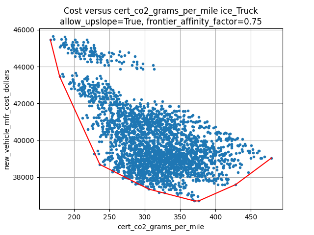
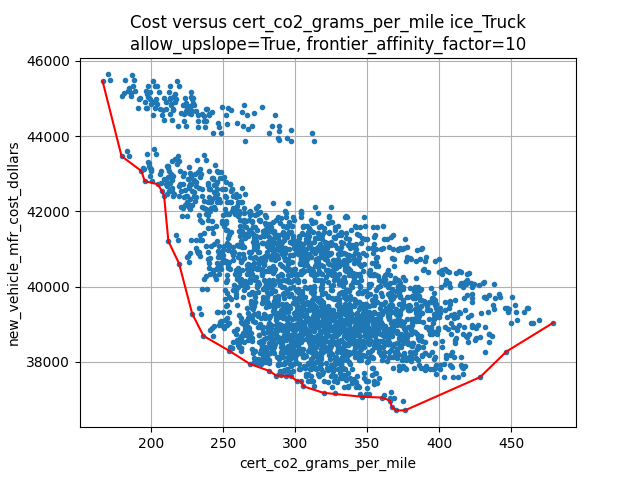
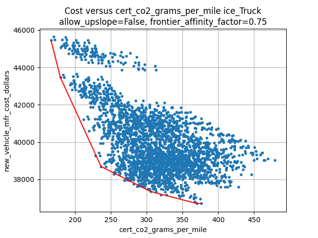
Each cost curve class includes multiple vehicles and represents the design space for all vehicle options in each class. In this example, multiple vehicles are grouped within a single cost curve class to reduce the number of simulations required to represent the design space. OMEGA producer decisions are made based on discrete vehicle options within each vehicle cost curve class. For possible future consideration, EPA recommends the generation of RSEs (response surface equations) to derive particular cost clouds unique to each vehicle. This would allow for more unique cost and vehicle clouds without excessive simulation calculation burden.
4.3.5. Vehicle Cost Clouds, Cost Curves, and Aggregation
The technology packages and their application to candidate vehicles are described in the model inputs as a discrete set of options that were generated using tools and approaches external to OMEGA (e.g. vehicle simulation, benchmarking, cost teardowns, etc.) Because the product design problem being solved is multi-dimensional (i.e. an intersection of technology package applications and market share decisions for multiple vehicles), the choice set must be built up from various combinations of vehicle-level decisions that cannot be readily predicted in advance.
The Producer Module uses an approach of aggregating the discrete, vehicle-level decisions at several levels, while retaining the vehicle-specific information that can be accessed later in other stages of the modeling and presented in the results. These processes of vehicle aggregation (also referred to as composition or the creation of “composite vehicles”) and decomposition are critical for the solution search process. First, aggregation allows the model to efficiently search for a solution without a complete enumeration of all possible choice combinations. Second, decomposition allows the model to draw upon the key vehicle attribute details that have been retained and are required for calculating the compliance emissions values and estimating the consumer response.
Vehicle-level technology application options
In oder to minimize cost, a producer would need to select the minimum cost package available at a given compliance emissions rate (i.e. g CO2/mi.) This subset of cost-minimizing vehicle technology packages is referred to as the cost curve, while the broader set of points is the cost cloud. Note that ‘cost’ here is referring to the producer generalized cost, as explained in Section 4.3.2.
Example: Vehicle cost clouds
An example cost cloud for a single vehicle in MY2025 (vehicle #62, a 4WD minivan) for the no-action policy in Context A is shown in Fig. 4.7. The costs for the blue points are production costs. The orange point costs are producer generalized costs, and include 5 years of fuel costs at 15,000 miles per year that the producer assumes are valued by consumers at the time of purchase (as defined in the analysis context input file ‘producer_generalized_costs.csv’.) Note that the producer generalized costs are higher than the production costs, and also form a cloud with a different shape than the blue production cost cloud. Essentially, the orange cloud is shifted up and rotated counterclockwise relative to the blue cloud because the technology packages with higher emissions rates also have relatively higher fuel costs that are assumed to factor into consumer purchases.
Fig. 4.7 also contains the resultant cost curve (black line) that represents the cost-minimizing frontier of the cost cloud. The Producer Module automatically generates this piece-wise linear approximation of the frontier using points in the cloud.
Compliance options based on design decisions across multiple vehicles
Because a producer can offer a range of different vehicles, each with distinct costs associated with applying technology packages, it is not likely that the lowest cost compliance solution will be a uniform application of technology to all vehicles. Nor will selecting the lowest cost option for each vehicle likely result in producer compliance, except in cases where a policy is non-binding. In order to consider design options for multiple vehicles simultaneously, the Producer Module aggregates individual vehicles into composites, with one composite vehicle for each market class and reg class combination. It is important that the resultant cost curves (producer generalized cost vs. g CO2/mi emissions rates) are not aggregated further since 1) aggregating emissions rates across market classes would no longer be valid after iteration when the Consumer Module changes the relative shares of market classes, and 2) aggregating emissions rates across regulatory classes would, under some policy definitions, make it impossible to calculate the Mg CO2 compliance credits (e.g. in policy cases where there are limits to the transfer of credits between regulatory classes.)
Example: Vehicle aggregation into market class - reg class cost curves
Fig. 4.8 shows the black cost curve of veh #62 as presented in Fig. 4.7, along with the other vehicles that are in the same combination of market class (ICE non-hauling) and reg class (‘a’.) Note that the simulated_vehicles.csv file for this example does not contain distinct costs and emissions rates for every vehicle. As a result, even though there are 12 vehicles are represented here, they overlay into only three distinct cost curves. If a user provided simulated_vehicles.csv inputs defined with greater resolution, every vehicle could be associated with its own distinct cost curve.
The bold orange line in Fig. 4.8 is the MY2025 cost minimizing frontier for a composite vehicle made by aggregating the individual vehicle cost curves in the same market class and reg class combination. The relative shares of vehicles within a market class and reg class remain fixed in the Producer-Consumer iteration process. Therefore the composite vehicle cost curve does not change as a result of the consumer response. This curve, along with the composite vehicle cost curves from the other market class and reg class combinations, is used to generate the producer compliance options.
Fig. 4.8 Example aggregation of vehicles into a composite vehicle
Once composite vehicle cost curves are generated for each market class and reg class combination, the Producer Module creates compliance options from a combination of design choices for the relative shares of composite vehicles and the emissions rate of each composite vehicle. The resulting compliance options are defined in terms of cost vs. Mg CO2 credits rather than g CO2/mi. See Section 4.5 (iteration and convergence) for more discussion of how the model converges on a solution by searching among these compliance options, and generating interpolated compliance options that are successively more refined with each iteration.
Extracting key vehicle attributes from the composite vehicles through decomposition
Once a compliance option is selected through the iteration and convergence process, a user will likely want to know how specific vehicle design decisions contributed to that solution.
Example: Decomposition of composite vehicle
Because the composite vehicle is made up of individual vehicles of fixed sales shares (at least relative to the other vehicles in the same market class, reg class combination), there is one-and-only-one solution for individual vehicle costs and emissions rates that will result in the selected option for the composite vehicle’s cost and emissions rate. Fig. 4.9 shows the same orange composite vehicle curve from Fig. 4.8, along with star symbols to indicate the selected option for the composite vehicle and associated points for the individual vehicles.
Fig. 4.9 Example decomposition of composite vehicle back to individual vehicles
The Consumer Module is a significant addition to OMEGA. With the ongoing evolutions in the light-duty vehicle market, including major growth in technologies and services, the need for an endogenous consumer response is clear. The Consumer Module is structured to project how consumers of light-duty vehicles would respond to policy-driven changes in new vehicle prices, fuel operating costs, trip fees for ride hailing services, and other consumer-facing elements. The module is set up to allow the inputs to affect total new vehicle sales (both in number and proportion of sales attributes to different market classes), total vehicle stock (including how the used vehicle market responds), and total vehicle use (the VMT of the stock of vehicles).
An important consideration with the addition of the Consumer Module is ensuring consistency between the set of vehicles and their attributes that the Producer Module supplies and the set of vehicles and their attributes that the Consumer Module demands. In order to estimate the set of new vehicles that provide this equilibrium, the Consumer and Producer modules iterate until convergence is achieved - where the set of vehicles, including their prices and attributes, that satisfy producers is the same set of vehicles that satisfy consumers.
As explained in the Overview chapter, and shown in Fig. 1.1, OMEGA is structured in a modular format. This means that each primary module — the Policy Module, Producer Module, Consumer Module and Effects Module — can be changed without requiring code changes in other modules. This ensures users can update model assumptions and methods while preserving the consistency and functionality of OMEGA.
An overview of the Consumer Module can be seen in Fig. 4.10. This overview shows the connections between the Consumer Module, the analysis context, and other OMEGA modules. The Consumer Module receives inputs from the analysis context and the Producer Module, and computes outputs used in iteration with the Producer Module and for use in the Effects Module.
The Consumer Module’s purpose is to estimate how light duty vehicle ownership and use respond to key vehicle characteristics within a given analysis context. There are five main user-definable elements estimated within the Consumer Module, as seen in Fig. 4.11. These estimates are: market class definitions, new sales volumes, new vehicle sales shares by market class (where market classes depend on the requirements of the specific consumer decision approach used in the analysis), used vehicle market responses (including reregistration), and new and used vehicle use measured using vehicle miles traveled (VMT). Further explanations of each of these elements are described in the following sections.
Each of these five elements represents a user-definable submodule within the Consumer Module code. The code within each submodule may be updated by a user, or the submodule may be replaced with an alternative submodule. When a modifies a submodule, they must ensure that the submodule retains consistency with the other submodules within the Consumer Module, as well as with the rest of OMEGA. For example, if the market class submodule is changed, the sales share submodule must be updated as well since sales shares are determined by market class.
The user-definable submodules of the Consumer Module in this example are listed in the table below.
Element
Submodule
Market class definitions
market_classes.py
New vehicle sales volume
sales_volume.py
New vehicle sales shares
sales_share.py
Used vehicle reregistration
reregistration_fixed_by_age.py
New and used vehicle use
annual_vmt_fixed_by_age.py
The Consumer Module works in two phases: first, an iterative new vehicle phase, followed by a non-iterative stock and use phase. During the first phase, the Consumer Module and Producer Module iterate to achieve convergence on the estimates of new vehicles produced and demanded that meet the standards set in the Policy Module. The Producer Module sends a set of candidate vehicles, including their prices and attributes, to the Consumer Module to consider. The Consumer Module uses that set of candidate vehicles to estimate total new vehicles demanded and the shares of those new vehicles in the specified market classes, which are passed back to the Producer Module. If the estimates do not converge within a tolerance, a new set of candidate vehicles is sent to the Consumer Module for consideration. See Section 4.5 for more information on the Consumer-Producer iteration process. Once convergence between the Producer and Consumer modules is achieved, the set of candidate vehicles are no longer considered candidates for consideration, but are the estimated new vehicle fleet, and the Consumer Module enters the second phase. In this phase, total vehicle stock (new and used vehicles and their attributes) and use (VMT) are estimated.
Inputs to the Consumer Module
In general, the Consumer Module uses exogenous inputs from the analysis context, and endogenous inputs from the Producer Module. The exogenous inputs may include data such as fuel prices, existing vehicle stock, and specific modeling parameters, for example, the parameters used in estimations of vehicle ownership and use decisions. The analysis context must also contain the inputs required to define projections of vehicle ownership and use in the absence of any policy alternatives being analyzed. These projections might be provided directly as inputs to the Consumer Module, such as projections of vehicle ownership from the Annual Energy Outlook (AEO), or generated within the Consumer Module based on exogenous inputs, including future demographic or macroeconomic trends. Endogenous inputs are factors determined within the model and passed to the Consumer Module from the Producer Module. They may include vehicle prices and other relevant vehicle attributes, such as fuel consumption rate. Because the Consumer Module’s internal representation of consumer decisions can be defined by the user, the specific exogenous and endogenous inputs required will depend on the models, methods, and assumptions specified by the user. The vehicle attributes needed as inputs to the Consumer Module are determined by the methods used to estimate new vehicle sales, the market shares of vehicles demanded, used vehicle reregistration, and new and used vehicle use. For example, vehicle attributes used to define market classes must be included as inputs from the Producer Module. As an additional example, if the user defines vehicle sales responses to differ based on consumer income, the user must ensure that income is included in the analysis context inputs.
Outputs of the Consumer Module
The Consumer Module produces two categories of outputs: sales estimates during the iterative Phase 1, and stock and use estimates during the non-iterative Phase 2. During the iterative phase, outputs of the Consumer Module, including new vehicle sales and responsive market shares (explained in the following section), are fed back to the Producer Module for iteration and convergence. See Section 4.4.3 for more information on what happens during Phase 1, and Section 4.5 for more detailed information on how OMEGA estimates iteration and convergence between the Producer and Consumer modules. Once that convergence is achieved, the Consumer Module estimates the outputs of the stock of vehicles, including both new and reregistered used vehicles, and VMT, which are used by the Effects Module.
During the iterative first phase, the Consumer Module considers vehicle prices and attributes at an aggregate level by grouping vehicles into market classes. These market classes are the fundamental unit of analysis for which the Consumer Module estimates new vehicle sales and shares. The choice of market classes is tied to the specification used to estimate the shares of new vehicles sold, and is dependent on the attributes available in the input data files. For example, vehicles might be identified by attributes such as fuel type (electric, gas, diesel, etc.), expected use (primarily for goods or passenger transport), or size.
Users can define market classes in the market class definitions submodule (as shown in Fig. 4.11.) In doing so, the user must ensure that all other inputs and user-definable submodules (for example, with respect to stock and use estimation) within the Consumer Module are defined consistently. For example, if the sales share submodule is defined as estimating shares of vehicles in a set of fuel type categories, those fuel type categories must be defined within the market class submodule.
The designation of market classes can be used to reflect market heterogeneity in purchasing behavior or vehicle use based on specific vehicle attributes. Accordingly, market classes are defined using vehicle attributes and inputs from the analysis context (i.e. the base year vehicle inputs.) In addition, the user can categorize market classes as ‘responsive,’ where the shares of total vehicles attributed to those market classes change due to endogenously modeled elements that change in response to policy (like relative costs), or ‘nonresponsive,’ where the shares of total vehicles attributed to those market classes do not change with the policy being analyzed.
Before the Consumer Module can estimate new vehicle sales or market shares responses, all vehicles must be categorized into their market classes. This categorization is defined as a series of nested market category levels. The user can define any number of market classes, or levels, as well as the hierarchy of the levels. In defining the hierarchy, it is important to note that OMEGA assumes that the sales share estimates within a parent category are independent of sales share estimates outside the parent category. This means that changing the available market classes outside the parent category will not change the sales share estimates within the parent category.
Example: Market class structure
Fig. 4.12 below illustrates the nested market class hierarchy used in this example. Hauling/non-hauling market classes are the highest, parent, level. Vehicles are separated into the appropriate hauling and non-hauling class using their attributes. Nested within the hauling and non-hauling categories, there are BEV/ICE market classes. The candidate vehicle inputs from the Producer Module, for example, vehicle prices, fuel cost and VMT, are used to determine the share of vehicles in the BEV/ICE market classes, as described in the examples below. During the iterative first phase, if the share of BEVs that consumers will accept given the candidate vehicle attributes does not converge within a tolerance with the share that the Producer Module estimates, the iterative process continues. The demanded BEV share is passed back to the Producer Module, which will return a new set of candidate vehicles and their attributes, including prices. Given the updated candidate vehicle inputs, the Consumer Module will redistribute vehicles into the BEV and ICE classes, with the BEV/ICE share estimates in the hauling category being independent from those in the non-hauling category. This possible redistribution between market class categories is represented by the dashed lines between each set of BEV/ICE classes. Note that the dashed lines travel within the hauling class and within the non-hauling class, but do not travel across them.
Fig. 4.12 Illustration of the Market Class Structure in the Example Analysis
Within a given analysis context, the shares of vehicles allocated to nonresponsive market class categories do not shift between those nonresponsive market categories, even under different policy alternatives or during iteration with the Producer Module. Shares of vehicles allocated to responsive market class categories may shift between the responsive market categories.
Example: Nonresponsive and responsive market classes
Within the example analysis, vehicles are separated into four market classes depending on whether they are categorized as hauling (primarily meant for transporting goods or towing, as a body-on-frame vehicle would be expected to do) or non-hauling (primarily meant for passenger transportation, as a unibody vehicle might do), and their fuel type (battery electric vehicle (BEV) or internal combustion engine vehicles (ICE)). The hauling/non-hauling market classes are defined as nonresponsive market class categories. The share of vehicles defined as hauling or non-hauling, regardless of the fuel type, depends on analysis context inputs, and is unaffected by model results. The BEV/ICE market classes are defined as responsive market class categories, the share of vehicles in that market class is estimated within the Consumer Module and is responsive to vehicle cost and fuel consumption rate of the set of candidate vehicles input from the Producer Module.
During the iterative first phase of the Consumer Module, the Producer Module and Consumer Module iterate to estimate total new vehicle sales, market shares, and prices at the market class level, based on the candidate vehicle options being offered by the producer. The iteration process is described more fully in the Iteration and Convergence Algorithms section. It begins with the Producer Module providing a set of candidate vehicles that meet the policy targets as defined within the Policy Module while minimizing the producer’s generalized costs. At this initial step, overall volumes are taken directly from the analysis context projections, along with sales shares projection of nonresponsive market class categories. If the sales and market shares result estimated within the Consumer Module is not within a given threshold of the estimates from the Producer Module, iteration between the modules occurs. The process entails the Producer Module offering successive sets of candidate vehicles and their attributes, including prices, which still achieve the policy targets until a there is set of candidate vehicles which results in agreement between the Producer Module and Consumer Module estimates of sales and market shares, or until an iteration limit is reached. On the Producer Module side, the process also includes determining the level of cross-subsidization between vehicle classes, which is covered more fully in the Iteration and Convergence Algorithms section. Within this iterative first phase of the Consumer Module, there are two main determinations being made: the total sales volume consumers will accept, and the share of vehicles they demand from each market class. Much of the method and assumptions used to estimate sales and shares impacts can be defined by the user in the New Vehicle Sales Volumes and New Vehicle Sales Shares submodule as seen in Fig. 4.11, including the method of estimating a change in sales volumes or responsive market shares, consumer responsiveness to price, and what is included in the price consumers take into account.
Sales volumes
The Consumer Module estimates the total new vehicles sold at the aggregated market class level with the user-definable submodule for new vehicle sales. The estimate for the change in new vehicle sales starts with an assumption of sales volumes in the Context Policy (the “no-action alternative”). These estimates can be an exogenous input from the analysis context, or estimated within the Consumer Module. Sales volumes under a defined policy (an “action alternative”) can be responsive to policy if the estimation is defined as relying, at least in part, on inputs from the Producer Module, or may be unresponsive to policy if the estimation is defined to rely solely on inputs from the analysis context. In defining how the Consumer Module estimates sales volumes, the user must ensure consistency between the inputs available from both the Producer Module and the analysis context, as well as with the other user-definable submodules within the Consumer Module. For example, if a user defines sales volumes as responsive to a specific vehicle attribute, that attribute must be included in the set of candidate vehicles and their attributes input from the Producer Module.
Example: New vehicle sales estimates
In the example analysis, sales volumes under the no-action policy alternative, which is also the Context Policy, are an exogenous input from the analysis context. An elasticity of demand, defined by the user, is used in conjunction with the change in price between a no-action alternative and an action alternative to estimate the change in sales from the no-action alternative level. Demand elasticity is defined as the percent change in the quantity of a good demanded for a 1% change in the price of that good, where the good demanded in the Consumer Module is new light duty vehicles. They are almost always negative: as the price of a good increases (a positive denominator), the amount of that good purchased falls (a negative numerator). Larger (in absolute value) negative values are associated with more “elastic”, or larger, changes in demand for a given change in price. This value represents how responsive consumers are to a change in price. The general elasticity equation is:
In the example analysis, the default elasticity of demand is set to -1. This means, for a 1% change in the consumer generalized price (described below), the vehicles demanded by consumers will fall by 1%.
In order to estimate the change in sales expected as function of the estimated change in price, this equation is rearranged:
At an aggregate level, the average expected change in the price of new vehicles is multiplied by the defined demand elasticity to get the estimated change in vehicles demanded. This change is combined with projected new vehicle sales under the no-action alternative to get the total new vehicle sales under the action alternative outlined in the Policy Module.
If a user adopts the example analysis method of estimating sales volumes using an elasticity of demand, they must ensure that net vehicle price, P, is defined. This net price is estimated under the no-action and the action alternatives, and the no-action alternative net price is subtracted from the action alternative net price to get an estimated change in net price, , that can be used with the user-specified elasticity. The net price should include factors the user assumes consumers consider in their purchase decision. Some factors that might be included are the share of total costs the producers pass onto the consumers, and the amount of future fuel costs consumers consider in their purchase decision.
Example: Net price
In the example analysis, the net price value in the sales volume estimate includes assumptions about the share of the total cost that producers pass onto the consumer and the amount of fuel consumption considered in the purchase decision. With respect to the share of total cost that producers pass onto consumers, this example assumes “full cost pass-through.” This means that the full increase in cost that producers are subject to in achieving emission reduction targets is passed on to the consumers. However, due to cross-subsidization, those costs may be spread across multiple market classes.
The role of fuel consumption in the purchase decision is represented by the number of years of fuel consumption consumers consider when purchasing a new vehicle, and can range from 0 through the full lifetime of the vehicle. Fuel costs are estimated using vehicle fuel consumption rates from the Producer Module, projections of fuel prices from the analysis context, the user-specified VMT schedules, and the user-specified vehicle reregistration schedules. The resulting portion of fuel costs considered by consumers is added to the candidate vehicle prices from the Producer Module to produce a net vehicle price, which is then used in conjunction with the elasticity of demand to estimate the change in vehicle sales. This example analysis assumes that consumers consider 5 years of fuel costs in the vehicle purchase decision.
Sales shares
The new vehicles sold are categorized into the user-definable market classes using estimates of sales shares. As mentioned above, those market classes can be nonresponsive or responsive to the policy being analyzed. Nonresponsive vehicle shares do not change with updated candidate vehicle sets or across policy alternatives. Though not responsive to endogenous inputs, the nonresponsive sales shares do not have to be constant. For example, they may be provided as a set of values for different points in time if the shares are expected to change exogenously over time. In addition, users can define sales shares to explicitly consider consumer heterogeneity by defining separate sales share estimates for different consumer groups. For example, sales share responses can differ between rural and urban consumers. If users identify heterogenous consumer groups with separate sales share responses, the analysis context must include the appropriate inputs. For example, the proportion of the vehicle buying population in urban and rural areas for each year being analyzed within the model.
Example: Nonresponsive market share estimates
Within the example analysis, the hauling/non-hauling market classes are nonresponsive. The sales shares for these classes are defined using exogenous inputs from the analysis context. The shares change over time as relative projections of hauling and non-hauling vehicles change over time. However, within a given analysis context, the shares do not change across the no-action and action alternatives defined in the Batch Input File.
For responsive market classes, users can define how market shares are responsive to attributes of candidate vehicle sets fed in from the Producer Module, for example vehicle price. In addition, the inputs used to estimate shares must be available within the set of candidate vehicles and their attributes, or as part of the analysis context.
Example: Responsive market share estimates
The example analysis defines BEV and ICE market classes as responsive to the action alternatives being analyzed. The method used to estimate BEV shares is based on an S-shaped curve, estimated using the logit curve functional form. Logit curves have been used to estimate technology adoption over time in peer reviewed literature as far back as 1957, and are still widely used today, including in estimating adoption of electric vehicle technologies. Technology adoption in a logit curve is modeled as a period of low adoption, followed by a period of rapid adoption, and then a period where the rate of adoption slows. This can be thought of as analogous to the “early adopter”, “mainstream adopter” and “laggard” framework in technology adoption literature. The logit curve equation in this example analysis estimates the share of BEVs demanded by consumers, accounting for how quickly (or slowly) new technology is phased into public acceptance, as well as how responsive consumers are to the candidate vehicle prices input from the Producer Module. The basic logit equation is:
is the share weight of market class i. This determines how quickly consumers accept new technology.
is the generalized cost of each vehicle in market class i
represents how sensitive the model is to price.
The table below shows a subset of input parameters used to estimate sales shares in this example analysis for Context A. Context B uses the same parameters with slightly different values.
Table 4.6 Example of Sales Share Parameters in ‘sales_share_params.csv’
market_class_id
start_year
annual_vmt
payback_years
price_amortization_period
share_weight
discount_rate
o_m_costs
average_occupancy
logit_exponent_mu
hauling.BEV
2020
12000
5
5
0.142
0.1
1600
1.58
-8
hauling.BEV
2021
12000
5
5
0.142
0.1
1600
1.58
-8
hauling.BEV
2030
12000
5
5
0.5
0.1
1600
1.58
-8
hauling.BEV
2031
12000
5
5
0.55
0.1
1600
1.58
-8
non_hauling.BEV
2020
12000
5
5
0.142
0.1
1600
1.58
-8
non_hauling.BEV
2021
12000
5
5
0.142
0.1
1600
1.58
-8
non_hauling.BEV
2030
12000
5
5
0.5
0.1
1600
1.58
-8
non_hauling.BEV
2031
12000
5
5
0.55
0.1
1600
1.58
-8
If the user retains the method of determining responsive BEV shares (using a logit curve as described above), the parameters representing the speed of acceptance, , and price responsiveness, , are factors the user can modify in the sales share submodule inputs (see salesshareinputs)
In addition, the user must specify the price used in the logit equation. This price should include factors the user estimates are significant in determining relative market shares; cost factors can be monetary, such as capital and maintenance costs, or non-monetary, such as time. In addition, price estimation needs to be consistent with the speed of acceptance and price responsiveness parameters.
Example: BEV share parameters
The share weight and price sensitivity parameters in this example analysis are currently informed by the inputs and assumptions used in the market share logit equation in the passenger transportation section of GCAM-USA (documentation and information on how to download GCAM-ISA can be found at https://jgcri.github.io/gcam-doc/gcam-usa.html ) In addition, the price used in estimating BEV shares is the consumer generalized cost used by the GCAM-USA share weight estimation method. The consumer generalized cost estimation from GCAM includes capital costs (including candidate vehicle prices fed in from the Producer Module, and the cost of a home charger), fuel costs, maintenance costs, and parameter values for amortization period and discount rate. The amortization period and discount rate, like most of the user-definable submodule, can be defined by a user. In this example, they are set at 10 years and 10%. These parameters are used to estimate an annualized vehicle cost. That annualized cost is then divided by a user defined annual vehicle mileage to convert the value to dollars per mile. Note that fuel costs are also included in GCAM’s generalized costs as $/mi, and are not discounted.
If convergence with respect to the sales and shares of new vehicles is achieved, the Consumer Module estimates total vehicle stock and use. To do so, it needs to keep internal consistency between- the number of vehicles demanded and the use of those vehicles. The method of determining total vehicle stock and vehicle use are in user-definable submodules represented by the used vehicle market response element and the new and used vehicle use element in Fig. 4.11. Vehicle stock is the total onroad registered fleet, including both new vehicles sales and the reregistered (used) vehicles. The data contained in the set of vehicle stock includes both vehicle count, as well as the attributes of the vehicles in the set, including model year and the vehicle features or attributes used to designate market classes. Vehicle use is the measure of how much each vehicle is driven in the analysis year, measured in vehicle miles traveled (VMT). VMT is determined at the vehicle level.
Vehicle stock
Fig. 4.13 below steps through the flow of how total vehicle stock is estimated in OMEGA. To estimate vehicle stock, the model starts with a base year stock of vehicles, which is an input from the analysis context. The base year is the last year actual observations, and is unmodified during the analysis. The analysis start year is the first year in which modeling is performed and immediately follows the base year. The stock of vehicles at the end of the analysis start year includes the new vehicles produced, plus the set of vehicles that were reregistered from the base year stock. For each subsequent modeled (analysis) year, the total stock is determined from the new vehicles produced in that year plus the reregistered vehicles from the prior year.
The method of estimating the reregistered fleet is in a user-definable used vehicle reregistration submodule. This method can make use of a static schedule, for example, where a vehicle’s age is the only determinant of the proportion of vehicles remaining in the fleet over time, or depend on other vehicle attributes, like cumulative VMT. If users modify the reregistration submodule to follow a different prescribed static rate, or to allow interdependencies between the rate of reregistration and other vehicle attributes, they need to retain consistency between the reregistration submodule and other submodules, for example the submodules estimating new vehicle sales and total VMT.
Example: Vehicle stock estimates
In this example analysis, the analysis start year stock of vehicles comes from the analysis context, and reregistration is estimated using fixed schedules based on vehicle age. For every calendar year, a specified proportion of vehicles in each model year is assumed to be reregistered for use in the following calendar year. In this fixed schedule, the proportion of vehicles of a given model year remaining in the registered stock (i.e. the survival rate) falls as the vehicles age. For example, in 2030, the proportion of the original MY 2025 vehicles remaining is larger than the proportion of MY 2015 vehicles remaining.
Vehicle use
Vehicle use is estimated as the vehicle miles traveled for each vehicle in the stock for the analysis year. This can be thought of as a measure of consumer demand for mobility. The method of estimating total VMT for the stock of vehicles is in a user-definable new and used vehicle use submodule. VMT can be estimated simply as a function of vehicle age, or may be a function of age, market class, analysis context inputs or more. Use could also include estimates of rebound driving. Rebound driving is estimated as the additional VMT consumers might drive as a function of reduced cost of driving.
Example: VMT estimates
In this example analysis, total VMT demanded is an input from the analysis context and is constant across policy alternatives. Total VMT demanded is combined with the initial stock of vehicles and their attributes from the analysis context to determine the proportion of VMT attributed to cohorts of vehicles separated by age and market class. For each calendar year, the total VMT projected in the analysis context is allocated across the internally estimated stock of vehicles using this fixed relationship. This method allows VMT per vehicle to change with the total stock of vehicles, while assuming that consumer demand for mobility is not affected by the action alternatives under consideration.
OMEGA finds a solution in each analysis year using iterative search algorithms. As shown in the process flow diagram in Fig. 4.2, the model uses two iterative loops; a Producer-Policy loop and a Producer-Consumer loop. For both loops, convergence criteria must be achieved within a specified tolerance for the simulation to proceed. This section describes those loops in more detail, with additional information from an example.
‘Producer-Policy’ Iteration: Compliance Search
The iteration process begins with a search for the vehicle design options and market class shares that minimize producer generalized costs and achieve the desired compliance outcome, independent of any feedback from the Consumer Module regarding vehicle demand. In this step, individual compliance options are built up, with each option fully defining the shares of each market class, and the technology package applications on each of the producer’s vehicles. From all these compliance options, up to a pair of points is selected which are closest, above and below, to the strategic GHG target (i.e. Mg CO2e.). If all points are under- or over-target then the point nearest to the target is chosen. The market shares and technologies of the selected point(s) become seed values for the next sub-iteration. In each successive sub-iteration, the search area becomes narrower while also covering the options with greater resolution. Finally, when a point falls below the convergence tolerance for Mg CO2 credits or the search range has fallen below a minimum tolerance, the closest point is selected as the compliance option for the initial compliance search.
Example: Initial compliance search
Fig. 4.14 shows the various sub-iterations for the initial compliance search in this example for 2025. The left figure shows a number of blue points for the 0th sub-iteration. The two low cost points nearest to 0 Mg CO2e credits form the basis for the search in the next sub-iteration. The right figure show all 15 sub-iterations (0th to 14th), including the points selected in the 0th sub-iteration (blue stars.) Note that the sub-iterations shown by the colored gradient scale have progressively lower costs, and more closely focused around 0 Mg CO2e. The selected compliance option from the initial Producer-Policy compliance search is shown by a single red star.
Fig. 4.15 is another view of the same search, with greater magnification around the selected production option and surrounding options which were not selected.
Fig. 4.15 Zoom in on producer’s initial compliance selection (2025_0)
‘Producer-Consumer’ Iteration: Market Shares and Pricing
After a purely cost-minimizing option is selected in the initial compliance search, the Producer Module provides the vehicle attributes and prices, at the market class level, for consideration by the Consumer Module. Within a given Producer-Consumer iteration loop, the vehicle design options are fixed. The search for a solution is based on consideration of various market class share and pricing options. Criteria for convergence include 1) the percent change in average total price, and 2) the difference in the producer and consumer market shares. To achieve convergence, both of these metrics must be close to zero, within the specified tolerance.
Example: Consumer-Producer iteration
Within a single Producer-Consumer iteration loop, vehicle designs are fixed, but pricing and market class shares vary. Fig. 4.16 shows the various components of the first Producer-Consumer iteration loop for 2025 in this example (Context A, no action policy alternative.)
The upper left panel shows the range of producer cross-subsidy price multiplier options. The full range of multipliers in the 0th sub-iteration are dark blue points, which then narrow in range over eight sub-iterations. The final range of multipliers is shown by the red points.
In the upper right panel, those same pricing options are shown in terms of absolute prices. While the multipliers applied to hauling and non-hauling vehicles cover a similar range of values, the lower absolute prices for non-hauling vehicles results in a range of prices that is somewhat narrower than the range for hauling vehicles.
The two convergence criteria are illustrated in the bottom two panels of Fig. 4.16 (share delta for hauling BEVs in the lower left panel, and average total price delta in the lower right panel.) In this Producer-Consumer iteration, the market class shares offered by the producer do not converge with the shares demanded by the consumer over the range of cross-subsidy pricing options available. This is visible in the lower left panel, since the 0.4% share delta value in the final sub-iteration does not meet the convergence criteria. If convergence had been achieved, the iteration process of this analysis year would be complete, and the produced vehicles would be finalized. Otherwise, the iteration will proceed, with a new consideration of vehicle design options offered by the Producer Module.
Repeat Iteration of ‘Producer-Policy’ and ‘Producer-Consumer’
If the prior round of iterations is unable to find a converged solution, the process will continue by repeating a series of Producer-Policy compliance searches and Producer-Consumer market share and pricing searches. The process is the same as in the initial iteration, with one exception: that the Producer-Policy compliance search will use the market shares from the prior iteration’s Producer-Consumer search.
These iterations are repeated until the market class share and average total price convergence criteria are met, and the compliance search is complete. Alternatively, if the number of Producer-Consumer iterations exceeds the set limit, then the sales and market shares from the last iteration are used. In this case, any deviation from the Producer’s strategic compliance target in that analysis year must be made up for through the use of banked credits. Finally, the produced vehicles are logged for consideration in the Consumer Module’s vehicle stock and use submodules, and in the Effects Module.
Example: First iteration beyond initial Producer-Policy and Producer-Consumer iterations
Fig. 4.17 shows the points considered in the compliance search in the first iteration (2025_1) following the initial iteration(2025_0). Similar to the initial iteration, each point represents a compliance option that is the result of a unique combination of candidate vehicle design choices and market class shares. Note that compared to Fig. 4.14, the points in Fig. 4.17 are more sparse since the market shares in this iteration have been constrained to the shares selected in the prior Producer-Consumer iteration.
Fig. 4.17 Compliance search iteration (2025_1) following initial iteration (2025_0)
Fig. 4.18 Zoom in on producer’s compliance selection (iteration 2025_1)
Fig. 4.19 is similar to Fig. 4.16, and represents the Producer-Consumer pricing and market class share search in a subsequent round of iteration, after the producer has revised the vehicle design options. Unlike the initial iteration, the range of cross-subsidy pricing flexibility is now sufficient to allow the convergence criteria to be met, as shown in the lower left and lower right panels.
In its primary function as a regulatory support tool, OMEGA’s modeled outputs are intended to inform the type of benefit-cost analyses used
in EPA rulemakings and other analyses. We would likely use many of OMEGA’s outputs directly in the analysis for a regulatory action. In other cases, OMEGA
produces values that might help inform other models like MOVES. The scope of OMEGA’s effects modeling includes estimating both monetized
or cost effects and physical effects. The Effects Module builds on the outputs of the Consumer and Producer modules along with the analysis
context inputs as shown in Fig. 4.20.
Key examples of physical effects that OMEGA will estimate:
Stock of registered vehicles, along with key attributes
VMT of registered vehicles
Tailpipe GHG and criteria pollutant emissions
Upstream (refinery, power sector) GHG and criteria pollutant emissions
Key examples of monetized effects that OMEGA will estimate:
Vehicle production costs
Vehicle ownership and operation costs, including fuel and maintenance
Other consumer effects
Impacts of criteria air pollutants
Impacts of greenhouse gas pollutants
Congestion, noise, and safety costs
The Effects Module generates: physical effects, cost effects, safety effects, benefits and social effects. In general, the cost effects and benefits output files build upon the physical effects output file in conjunction with several of the context input files. Those context input files are the cost factors, vehicle emission rate inputs and upstream emission source data files. For example, the benefits file would present CO2-related benefits as the CO2 cost factor (a social cost of GHG per metric ton value set in the input file) multiplied by the emission impacts of CO2 (or other GHG) calculated using physical effects. Similarly, fuel costs would be calculated as fuel prices (dollars/gallon as provided in the input file) multiplied by gallons consumed as presented in the physical effects file.
One attribute appears in both the cost effects and the benefits files. That attribute is the drive value which is the economic value of the increased owner/operator surplus provided by added driving and is estimated as one half of the product of the decline in vehicle operating costs per vehicle-mile and the resulting increase in the annual number of miles driven via the rebound effect, plus the cost of driving those rebound miles. Since the drive value is calculated using a change in operating costs, the new operating costs must be compared to another operating cost. Drive value is calculated as a cost and presented in the cost effects file as the drive surplus plus the fuel costs associated with driving any rebound miles. Drive value is then calculated as a
benefit by calculating the drive value cost in an action scenario relative to the no-action scenario. If the drive value cost is greater in the action scenario, a positive drive value benefit will be the result while a lower drive value cost in the action scenario would represent a negative benefit, or disbenefit.
Importantly, the cost factor inputs (as OMEGA calls them) have been generated using several discount rates. The values calculated using each of the different discount rates should not be added to one another. In other words, PM costs calculated using a 3 percent discount rate and a 7 percent discount rate should never be added together. Similarly, climate costs calculated using a 3 percent discount rate and a 2.5 percent discount rate should never be added. This does not necessarily hold true when adding criteria air pollutant costs and climate costs when it is acceptable to add costs using different discount rates. Lastly, when discounting future values, the same discount rate must be used as was used in generating the cost factors.
The default effects files are annual summary results by calendar year, regulatory class and fuel type. If desired, vehicle-level output files can be selected via the RUNTIME OPTIONS portion of the effects batch file. The vehicle-level output files can be very large depending on the number of vehicles, length of vehicle life and number of calendar years included in the run. Files can be saved in a compressed ‘parquet’ format for use with Python’s pandas library to minimize file sizes, however, the parquet format is available only when running via OMEGA code and not when running via an executable bundle.
Note that the effects module is a separate runtime process from the producer and consumer processes discussed above. The effects module can be run from code by running omega_effects_main.py or by running the exectuable file. Either way, the user will be prompted to select the desired batch file for the run.
Physical effects are calculated at the vehicle level for all calendar years included in the analysis. Vehicle_ID and VMT driven by the given vehicle are pulled from the VehicleAnnualData class. Vehicle attributes are pulled from Vehicle class. Fuel attributes are pulled from the OnroadFuel class which draws them from the onroad_fuels input file.
is calculated within OMEGA and accounts for any credits that do not improve fuel consumption and test-to-onroad gaps
is the efficiency of the energy transfer from the charge point to the battery as set by the user
Note
Multi-fuel vehicle fuel consumption
Multi-fuel vehicles consume both electricity and liquid fuel. Consumption of both is calculated for such vehicles and emission effects such
as upstream and vehicle emissions are calculated uniquely for both fuels.
Cost effects are calculated at the vehicle level for all calendar years included in the analysis and for, primarily,
the physical effects described above.
Benefits are calculated at the fleet level by calendar year and are calculated based on the changes in physical effects relative to the no-action scenario specified in the batch settings input file for the effects run.
The primary input to OMEGA is the batch definition file which contains rows for each user input required to define a simulation session or group of sessions.
The line-by-line documentation of the batch definition file is available at omega_model/omega_batch.py and won’t be repeated here.
Batch definition inputs can be scalar values or input file paths (relative to the location of the batch file and/or absolute).
Several of the input files may dynamically load user-definable modules at runtime. These files are indicated as user_definable in the table below. User-definable inputs and modules are loaded by interpreting the input file input_template_name: field. For example, if the input template name of a user-definable input is consumer.market_classes then the Python module omega_model/consumer/market_classes.py will be used to load the rest of the input file, which may contain an arbitrary format known to the module. The process of creating user-definable modules is a topic for developers.
Below is a table with links to the modules that load the files and their documentation of the input file formats.
The context inputs apply to all sessions within a batch. Multiple batch files must be defined to run multiple contexts.
Simulation Sessions
The Context Session
The batch file must define at least one simulation session, known as the context session, which is the left-most session in the batch definition file. The context session should align with the provided context inputs. For example, if the context fuel price and new vehicle market data are from AEO, then the policy inputs of the reference session must be consistent with the assumptions used by AEO to generate the projections. For example, the sales projections take into account ghg and fuel economy policies in force or projected at the time and the policy inputs used for the context session should be consistent with those. It would be inconsistent to assume the same sales for a different ghg/fuel economy policy.
Policy Alternative Sessions
Optionally, one or more alternative policy sessions may be defined in subsequent columns. Typically these would be various policies under evaluation via OMEGA or perhaps a single policy with various alternative inputs or assumptions.
OMEGA Batch Command Line Interface
The batch process can be initiated from the OMEGA GUI or from the command line by running omega_batch.py directly, as in:
In fact, the GUI can be thought of as a wrapper to a command line call to omega_batch.py. The paths supplied to the GUI fill in the --bundle_path and --batch_file arguments.
Typical Command Line Usage (not all available command-line options shown)
usage: omega_batch.py
        [-h] [--bundle_path BUNDLE_PATH] [--batch_file BATCH_FILE]  [--ui_batch_file]
        [--session_num SESSION_NUM] [--analysis_final_year ANALYSIS_FINAL_YEAR]
        [--verbose] [--show_figures]

Run OMEGA batch simulation

optional arguments:
  -h, --help            show this help message and exit

  --bundle_path BUNDLE_PATH
                        Path to bundle folder

  --batch_file BATCH_FILE
                        Path to batch definition file

  --ui_batch_file
                        Select batch file from dialog box

  --session_num SESSION_NUM
                        ID # of session to run from batch

  --analysis_final_year ANALYSIS_FINAL_YEAR
                        Override analysis final year

  --verbose             Enable verbose omega_batch messages
Other command line arguments are available, mostly associated with parallel processing options and implementation or code development. The full list of arguments can be viewed as follows:
>>python omega_model/omega_batch.py

or

>>python omega_model/omega_batch.py -h

or

>>python omega_model/omega_batch.py --help
Selecting Sessions to Run
Sessions can be enabled or disabled within the batch file by setting the EnableSession field to TRUE or FALSE, respectively. Alternatively, the --session_num argument can be passed to omega_batch. The reference session is session number 0. The reference session cannot be disabled, regardless of the EnableSession field value, as it generates reference vehicle prices that the other sessions require in order to calculate overall vehicle sales.
Understanding the Batch Process
The first step in the batch process is to copy the complete source code to the bundle folder (in the omega_model directory, or as specified by the user via the --bundle_path argument) and to create subfolders for each active session. Within each session folder will be an in folder (and an out folder will be created when the session runs). The bundle folder contains the original batch definition file as well as a timestamped batch definition file that is actually run. The timestamped file has the original batch settings with new session input file paths relative to the bundle. The bundle folder contains a requirements.txt file for reference. When running from source code the requirements file indicates the version of Python used to run the batch and contains the list of installed Python packages and their versions at the time, e.g. python_3_8_10_requirements.txt. When running from the executable the contents of the GUI_requirements.txt file indicates the version number of the GUI.
The batch itself and each session will have a log file indicating the progress and success or failure of the process. The batch log file is named batch_logfile.txt and exists at the top of the bundle folder. Session logs have the prefix o2log_ and are located in each session’s out folder.
If a session completes successfully, the session folder is renamed and prepended with an underscore, _. Failed session folders are prepended with #FAIL_. In this way the session status can be monitored by observing the folder names as the batch runs.
Since the bundle folder contains the source code and all inputs for every session it is possible to re-run a batch, or part of a batch, at a later time and reproduce the results if desired. To do so, remove any session folder prefixes and use omega_batch.py to re-run the timestamped batch file, while supplying the --no_bundle and --no_validate arguments, since the batch has already been bundled. As in:
The primary inputs to the OMEGA effects calculator are the OMEGA Model’s vehicles and vehicle annual data output files for
sessions of interest. For the Effects calculator to find these necessary OMEGA Model output files, the user must provide to the
Effects calculator the path where they can be found. This is done via the effects batch input file. Assuming the user has run the OMEGA
Model and has the bundled results saved to an accessible directory, then the effects batch input file should provide the full system
path to that directory.
Importantly, the effects batch input file must also provide a session name associated with each session for which effects
are to be calculated. The session name must be consistent with the session name used in the OMEGA Model run. These session names
also need to include a context session name, a no action session name and at least one action session name. These are needed
to calculate the effects properly since the context session serves to calculate fleet vehicle miles traveled (VMT) and fleet fuel costs per
mile from which any VMT rebound effects in subsequent sessions can be calculated.
The OMEGA effects calculator will look for several necessary files within the “in” folder of the context session folder contained within the
bundled OMEGA Model results (i.e., the user need not specify these files in the effects batch input file). In addition to the context session,
a no action and action session are required because some of the effects calculations are meant to calculate impacts of a policy action relative
to a no action, or business as usual, policy. In particular, the benefits calculations can only be done by first calculating physical effects
of the action policy relative to the no action policy since benefits do not exist, within OMEGA, absent a policy change.
The other inputs to the OMEGA effects calculator are those associated with: vehicle emission rates; EGU and refinery data; cost factors
associated with criteria air pollutants, GHG emissions, energy security impacts, crashes, congestion, noise, vehicle repair, vehicle
maintenance, fuel prices, etc. All of these input files must be provided by the user via the effects batch input file.
Below is a table describing the entries needed in the effects batch input file. User entries are to be made in the
value or full_path columns of the effects batch input file.
Batch Input Files and Loaders
parameter
session_policy
description
RUNTIME OPTIONS
Run ID
all
enter value for the run identifier for your output folder name or blank for default (default is omega_effects)
Run Description
optional only to help the user identify the purpose of the run
Save Path
all
enter fullpath of the folder to which to save results but do not include unique run identifiers
Save Input Files
all
enter value as True to save input files to your results folder or False to save space and not do so
Save Context Fuel Cost per Mile File
all
enter value as True or False and note that these files can be large especially in CSV format
Save Vehicle-Level Safety Effects Files
all
enter value as True or False and note that these files can be large especially in CSV format
Save Vehicle-Level Physical Effects Files
all
enter value as True or False and note that these files can be large especially in CSV format
Save Vehicle-Level Cost Effects Files
all
enter value as True or False and note that these files can be large especially in CSV format
Format for Vehicle-Level Output Files
all
enter value as ‘csv’ for large Excel-readable files or ‘parquet’ for compressed files usable in Pandas (value must be csv when running executable)
Powertrain Costs FEV
all
enter value as True to use FEV developed cost curves
BATCH SETTINGS
batch_folder
all
enter full_path of the folder containing OMEGA Model run results
Vehicles File Base Year
all
enter value consistent with the OMEGA Model run
Analysis Final Year
all
enter value <= the value used in the OMEGA Model run
Cost Accrual
all
enter value as start-of-year or end-of-year - this entry impacts the discounting of costs and benefits
Discount Values to Year
all
enter value to which costs and benefits will be discounted
Analysis Dollar Basis
all
enter value consistent with the OMEGA Model run
Context Name Liquid Fuel
all
enter value of the AEO report (e.g. AEO2021) used in the OMEGA Model run
Context Case Liquid Fuel
all
enter value of the AEO case (e.g. Reference case) used in the OMEGA Model run
Electricity Prices
all
enter value to specify which electricity prices to use for No Action and Action session effects (e.g.
IPM or AEO)
VMT Rebound Rate ICE
all
enter value for ICE rebound (e.g. -0.1)
VMT Rebound Rate BEV
all
enter value for BEV rebound
SC-GHG in Net Benefits
all
enter value as ‘global’ or ‘domestic’ or ‘both’ (note that both global and domestic benefits are calculated
if available
this only impacts net benefits)”
Maintenance Costs File
all
enter full_path of maintenance costs file in CSV format
Repair Costs File
all
enter full_path of repair costs file in CSV format
Refueling Costs File
all
enter full_path of refueling costs file in CSV format (i.e. the cost of time spent refueling)
General Inputs for Effects File
all
enter full_path of general inputs for effects file in CSV format
Criteria Cost Factors File
all
enter full_path of criteria air pollutant $/ton factors file in CSV format
SCGHG Cost Factors File
all
enter full_path of social cost of GHG $/ton factors file in CSV format
Energy Security Cost Factors File
all
enter full_path of energy security $/barrel file in CSV format
Congestion-Noise Cost Factors File
all
enter full_path of crashes & congestion & noise costs file in CSV format
Insurance and Taxes Cost Factors File
all
enter full_path of insurance and taxes cost file in CSV format
Legacy Fleet File
all
enter full_path of legacy fleet file in CSV format
CPI Price Deflators File
all
enter full_path of CPI price deflators file in CSV format
EGU Data File
all
enter full_path of EGU data file in CSV format
Refinery Data File
all
enter full_path of Refinery data file in CSV format
Safety Values File
all
enter full_path of safety values file in CSV format
Fatality Rates File
all
enter full_path of fatality rates file in CSV format
SESSION SETTINGS
Session Name
context
enter value of the context session name
Context Stock and VMT File
context
enter full_path of stock and VMT file file in CSV format
Context Electricity Prices
context
enter full_path of electricity prices file used for the context session
Session Name
no_action
enter value of the No Action session name
Session Vehicle Emission Rates File
no_action
enter full_path of vehicle emission rates file in CSV format used for the No Action session
Context Electricity Prices
no_action
enter full_path of electricity prices file in CSV format used for the No Action session
Session Name
action_1
enter value of the Action session name
Session Vehicle Emission Rates File
action_1
enter full_path of vehicle emission rates file in CSV format used for the Action session
Context Electricity Prices
action_1
enter full_path of electricity prices file in CSV format used for the Action session
The effects results will be saved to a folder specified in the save_path full_path entry (e.g. “c:/omega/effects”). In that save_path folder,
a folder will be auto generated and will have the same name as the OMEGA Model batch for which effects are being calculated.
Within that batch folder, a run results folder will be auto generated whose name will consist of a date and timestamp associated with
the time of the OMEGA effects calculator run along with the run ID to assist in keeping track of different runs and ensuring that nothing is
overwritten by future runs. As a result, you might find your results saved to a folder named something like
“c:/omega/effects/ld_omega_model_batch/20230504_090000_omega_effects” for a run done on May 4, 2023, at 9:00AM.
Note that some effects output files may or may not be desired. The effects are calculated for every vehicle in the fleet in every
year up to and including the Analysis Final Year value. If you run through 2055, this becomes a large number of vehicles and
the vehicle-level output files can become very large (0.5 GB to 1 GB per file). Depending on your machine, you may have trouble
viewing those files let alone conducting analyses of the results (e.g., in Excel or OpenOffice). Saving of these large output files
can be avoided by setting the “Save Vehicle-Level” file value to False. Alternatively, the user can generate those files in
parquet format, which is a compressed file format, to save space. Parquet files are readable by Python’s Pandas library but cannot
be opened directly in a spreadsheet application. Instructions for reading saved parquet files in Pandas are included in the save_file function
of /omega_effects/general/file_id_and_save.py. Note that saving to parquet format only works
when running from the OMEGA code, and that the selection must be set to ‘csv’ format when running from the executable.
Any session can be run in the OMEGA Effects calculator provided those sessions exist in the batch_folder. A value for
the session name must be provided. A session can be ignored by setting the Session Name value to None. A Context Session Name
must be provided and no session meant to be included can have a session name of None.
Note that an action session may require a different emission rate input file than that used for the no action session for, say,
vehicle emission rates in the event that the policy impacts vehicle emission rates.
The OMEGA Effects are not part of the OMEGA Model executable file. The OMEGA Effects can be run using the Python code included in the OMEGA repository at https://github.com/USEPA/EPA_OMEGA_Model or the Python code included in the zip file available at the OMEGA webpage linked above.
Alternatively, the OMEGA Effects can be run using a separate executable file available on the OMEGA webpage (recommended).
These instructions assume that the executable file is being used to generate the OMEGA Effects.
Place the executable file in your preferred location on your local machine.
Place the inputs files in your preferred location on your local machine.
Find a copy of the effects batch settings file.
In cell C3 of the batch settings file, enter a run ID if desired (e.g., My_run, test, etc.). This run ID will be included as part of the output folder name. The default value is omega_effects.
In cell D5, enter the path of the save folder (e.g., “C:/omega/effects”). The output folder will be saved to this folder. The output folder will be named using other entries in the batch file and the run ID set in step 8.
Other options in Column C can be set to TRUE or FALSE, but please read the notes associated with each.
In cell D14 of the batch settings file, enter the full path to the folder that contains your OMEGA compliance run results. This is important since the OMEGA Effects will look to this folder to find the needed vehicles.csv and vehicle_annual_data.csv files generated for each session in your OMEGA compliance run.
Most values in column C can be left as is. There must be a context session name in cell C42. If your context session name is different, then set cell C42 accordingly. The same is true of subsequent session names in column C. If you do not want your effects outputs to include a session that exists in your OMEGA compliance run folder, simply set the session name to None.
Remaining entries in Column D should then point to the inputs folder on your local machine. Filenames can probably be left as is unless you are using files with different names.
After setting up the batch settings file, be sure to save it as a CSV file (not Excel).
Double click the executable file.
The executable should launch. Be patient. After several seconds, a file dialog window should open asking for the batch settings file. Navigate to the batch settings file you saved in step 14, select it, and click open. The executable should now run using the settings in your batch settings file.
This Developer Guide will assist those interested in the latest (pre-release) version of OMEGA available from source code. This guide assumes some familiarity with Python programming and development, but also attempts to point newcomers in the right direction where possible.
The developer branch contains in-development, pre-release code, subject to change without notice and no guarantees as to stability at any given point in time. Features may be added or removed and may or may not be used for future rulemakings.
Releases will be available on separate branches that contain only the particular release in question.
OMEGA has been developed with Python versions 3.7.1 (the minimum required version) thru 3.11.6 and has not been tested with version 3.12 or higher. If you already have Python installed, there is probably no reason to update to a newer version unless one of the required packages is not compatible with your Python version and hardware platform.
The recommended practice is to run the source code in a virtual environment, which may be set up manually or via the IDE. The virtual environment isolates the installation of OMEGA-required Python packages from whatever packages may have already been installed at the system level. This allows a ‘clean’ installation that can guarantee no known conflicts between packages.
The simplest way to install the packages is to use pip, the package installer for Python. Sometimes there is an updated version of pip available. The command-line code below updates pip and installs the packages detailed in requirements.txt.
The primary use case for running omega.py directly is just to confirm the installation or perhaps when it’s simpler to debug code without the overhead of the batch process.
To run the gui directly from source at the command line from the project top-level folder:
Routines to load and provide access to annual vehicle miles travelled (VMT) by market class and age.
The data represents a fixed VMT schedule by age.
INPUT FILE FORMAT
The file format consists of a one-row template header followed by a one-row data header and subsequent data
rows. The template header uses a dynamic format.
The data represents the re-registered proportion of vehicles by calendar year, age and market class.
File Type
comma-separated values (CSV)
Template Header
input_template_name:
[module_name]
input_template_version:
[template_version]
Sample Header
input_template_name:
consumer.annual_vmt_fixed_by_age
input_template_version:
0.2
Sample Data Columns
start_year
age
market_class_id
annual_vmt
2019
0
non_hauling.BEV
14699.55515
2019
1
non_hauling.BEV
14251.70373
2019
2
non_hauling.BEV
14025.35397
2019
0
hauling.ICE
15973.88982
2019
1
hauling.ICE
15404.1216
2019
2
hauling.ICE
14840.93011
start_year:
Start year of annual VMT data, values apply until the next available start year
age:
Vehicle age, in years
market_class_id:
Vehicle market class ID, e.g. ‘hauling.ICE’
annual_vmt:
Vehicle miles travelled per year at the given age for the given market class ID
The file format consists of a one-row template header followed by a one-row data header and subsequent data
rows. The template header uses a dynamic format.
The data represents the re-registered proportion of vehicles by model year, age and market class.
File Type
comma-separated values (CSV)
Template Header
input_template_name:
[module_name]
input_template_version:
[template_version]
Sample Header
input_template_name:
consumer.reregistration_fixed_by_age
input_template_version:
0.2
Sample Data Columns
start_model_year
age
market_class_id
reregistered_proportion
1970
0
non_hauling.BEV
1
1970
1
non_hauling.BEV
0.987841531
1970
2
non_hauling.BEV
0.976587217
1970
0
hauling.ICE
1
1970
1
hauling.ICE
0.977597055
1970
2
hauling.ICE
0.962974697
Data Column Name and Description
start_model_year:
The start vehicle model year of the re-registration data, values apply until next available start year
Routines to load and access electricity prices from the analysis context and the sessions
INPUT FILE FORMAT
The file format consists of a one-row data header and subsequent data rows.
The data represent electricity charging costs per kWh.
File Type
comma-separated values (CSV)
Sample Data Columns
context_id
dollar_basis
case_id
fuel_id
calendar_year
retail_dollars_per_unit
pretax_dollars_per_unit
AEO2020
2019
Reference case
US electricity
2019
0.12559407
0.10391058
AEO2020
2019
Reference case
US electricity
2020
0.1239522
0.10212733
Data Column Name and Description
context_id:
The name of the context source, e.g. ‘AEO2020’, ‘AEO2021’, ‘IPM’, etc
dollar_basis:
The dollar basis of the fuel prices. Note that this dollar basis is converted in-code to ‘analysis_dollar_basis’
using the implicit_price_deflators input file.
case_id:
The name of the case within the context, e.g. ‘Reference Case’, ‘High oil price’, for AEO; ‘action’ or
‘no_action’ for IPM
fuel_id:
The name of the vehicle in-use fuel, must be in the table loaded by classfuels.Fuel and consistent with
the base year vehicles file (column in_use_fuel_id) loaded by classvehicles.VehicleFinal
Routines to load and access liquid fuel prices from the analysis context
Context fuel price data includes retail and pre-tax costs in dollars per unit (e.g. $/gallon)
INPUT FILE FORMAT
The file format consists of a one-row template header followed by a one-row data header and subsequent data
rows.
The data represents fuel prices by context case, fuel type, and calendar year.
File Type
comma-separated values (CSV)
Sample Header
input_template_name:
context_fuel_prices
input_template_version:
0.2
Sample Data Columns
context_id
dollar_basis
case_id
fuel_id
calendar_year
retail_dollars_per_unit
pretax_dollars_per_unit
AEO2020
2019
Reference case
pump gasoline
2019
2.665601
2.10838
AEO2020
2019
Reference case
US electricity
2019
0.12559407
0.10391058
Data Column Name and Description
context_id:
The name of the context source, e.g. ‘AEO2020’, ‘AEO2021’, etc
dollar_basis:
The dollar basis of the fuel prices in the given AEO version. Note that this dollar basis is
converted in-code to ‘analysis_dollar_basis’ using the implicit_price_deflators input file.
case_id:
The name of the case within the context, e.g. ‘Reference Case’, ‘High oil price’, etc
fuel_id:
The name of the vehicle in-use fuel, must be in the table loaded by classfuels.Fuel and consistent with
the base year vehicles file (column in_use_fuel_id) loaded by classvehicles.Vehicle
input_df (DataFrame) – the maintenance_cost_inputs.csv file with costs updated to analysis_basis_dollars.
Returns:
A dictionary of maintenance cost curve coefficients (slope with intercept=0)
having keys of ‘ICE’, ‘HEV’, ‘PHEV’, ‘BEV’.
Notes
Dividing the cumulative_cost by miles gives a constant cost/mile for every mile. However, costs/mile should
be lower early and higher later, so this method determines a triangular area that equates to the cumulative
cost. With the slope of that triangular area, a cost/mile at any odometer value can be calculated and the
cost of maintenance in any year can then be calculated as that cost/mile multiplied by miles driven in that
year.
This omega_effects module reads the powertrain cost file used in the compliance run for the given session for the sole
purpose of determinining the battery offset. The SessionSettings class searches for the applicable powertrain cost
file for the given session so the user need not worry about the powertrain cost file for effects calculations.
veh_cost – (Numeric) The value of the vehicle when sold as new
pt_type – (str) The powertrain type (ICE, HEV, PHEV, BEV)
repair_type – (str) The vehicle repair type (car, suv, truck)
age – (int) The age of the vehicle where age=0 is year 1 in operation
Returns:
A single repair cost per mile for the given vehicle at the given age
Note
The source data included MSRP up to $100,000 and through 10 years of service; MSRP is limited here to
$100,000 but calculations continue beyond 10 years at the growth indicated by the source data.
batch_settings – an instance of the BatchSettings class.
annual_physical_effects_df (DataFrame) – a DataFrame of physical effects by calendar year, reg class, fuel type.
annual_cost_effects_df (DataFrame) – a DataFrame of cost effects by calendar year, reg class, fuel type.
calc_health_effects (bool) – pass True to use $/ton values to calculate health effects. If cost_factors_criteria.csv
values (contains benefit per ton) –
False. (calc_health_effects will be True; blank values will result in the default) –
Returns:
one of benefits for each action session relative to the no_action session; and one of physical
effects for each action session relative to the no_action session.
A series of functions to calculate costs associated with the policy. The calc_cost_effects function is called by the
omega_effects_main module and other functions here are called from within the calc_cost_effects function.
batch_settings – an instance of the BatchSettings class.
session_settings – an instance of the SessionSettings class.
session_fleet_physical – A dictionary of physical effects for each vehicle in each analysis year.
context_fuel_cpm_dict – dictionary; the context session fuel costs per mile by vehicle_id and age.
Returns:
A dictionary of cost effects for each vehicle in each analysis year.
Notes
The average purchase price will include possible battery tax credits and reflects the expected price of a
vehicle on the dealer lot. The average price modification reflects possible purchase tax credits which would
be deducted from the average purchase price to reflect out-of-pocket purchase costs. Insurance, sales taxes,
and any other cost tied to the value of a vehicle use the average purchase price in applicable calculations. An
exception to that would be repair costs which are tied to the manufacturer cost and not purchase prices. The
manufacturer cost excludes cost reductions via applicable battery tax credits.
The file format consists of a one-row template header followed by a one-row data header and subsequent data
rows.
The data represents $/mile cost estimates associated with congestion and noise associated with road travel.
File Type
comma-separated values (CSV)
Sample Header
input_template_name:
cost_factors_congestion_noise
input_template_version:
0.1
Sample Data Columns
reg_class_id
dollar_basis
congestion_cost_dollars_per_mile
noise_cost_dollars_per_mile
car
2018
0.063390239
0.000940863
truck
2018
0.056598428
0.000940863
Data Column Name and Description
reg_class_id:
Vehicle regulatory class at the time of certification, e.g. ‘car’,’truck’. Reg class definitions may differ
across years within the simulation based on policy changes. reg_class_id can be considered a ‘historical’
or ‘legacy’ reg class.
dollar_basis:
The dollar basis of values within the table. Values are converted in-code to ‘analysis_dollar_basis’ using the
implicit_price_deflators input file.
congestion_cost_dollars_per_mile:
The cost per vehicle mile traveled associated with congestion.
noise_cost_dollars_per_mile:
The cost per vehicle mile traveled associated with noise.
The file format consists of a one-row template header followed by a one-row data header and subsequent data
rows.
The data represents $/uston benefits estimates associated with reductions in criteria air pollutants. The data should
be left blank to avoid calculating health effects (criteria air pollution effects) using $/uston values.
File Type
comma-separated values (CSV)
Sample Header
input_template_name:
cost_factors_criteria
input_template_version:
0.5
Sample Data Columns
calendar_year
dollar_basis
source_id
rate
study
pm25
sox
nox
2020
2020
car pump gasoline
0.03
Wu
0
0
0
2025
2020
car pump gasoline
0.03
Wu
709156.4844
127863.083
7233.620573
2030
2020
car pump gasoline
0.03
Wu
813628.2611
146570.4771
8157.897937
2035
2020
car pump gasoline
0.03
Wu
938850.3917
169075.4785
9195.259845
2040
2020
car pump gasoline
0.03
Wu
1060686.72
191135.9472
10073.96999
2045
2020
car pump gasoline
0.03
Wu
1171439.061
211302.6049
10731.06062
2050
2020
car pump gasoline
0.03
Wu
1268468.809
229133.7696
11165.95105
Data Column Name and Description
calendar_year:
The calendar year for which specific cost factors are applicable.
dollar_basis:
The dollar basis of values within the table. Values are converted in-code to ‘analysis_dollar_basis’ using the
cpi_price_deflators input file.
source_id:
The source of the pollutant, whether it be a gasoline car or an EGU or refinery.
rate:
The discount rate used in generating the $/ton benefits values.
The DiscountingBenefits class discounts annual values, sums those to calculate present values and annualizes those
present values for equivalent annualized values.
The discount_annual_values function determines attributes appropriate for discounting and does the discounting
calculation to a given year and point within that year.
Parameters:
batch_settings – an instance of the omega effects batch settings class.
annual_values_df (DataFrame) – including values to be discounted.
effects_log – an instance of the EffectsLog class.
Returns:
A dictionary providing discounted annual values where monetized values are discounted at their internally
consistent discount rate.
Note
Important input settings for discounting of monetized values are the “Discount Values to Year” and
“Cost Accrual” settings. The year to which to discount monetized values is set by the “Discount Values to
Year” entry of the omega effects batch input file. The “Cost Accrual” input setting should be set to
‘start-of-year’ or ‘end-of-year’, where start-of-year represents costs accruing at time t=0 within the
year, and end-of-year represents costs accruing at the end of the year.
Values that occur prior to the “Discount Values to Year” input setting will not be discounted.
Criteria health benefits are generated using $/ton inputs for criteria cost factors. Annual discounted values
calculated here are valid only for those social discount rates that match the discount rate used in
generating the $/ton benefit values. In other words, annual discounted values using a 2 percent social
discount rate are not valid if calculated using a 3 or 7 percent discount rate in generating the $/ton
values. That said, this does calculate those values for use in generating present and annualized values of,
for example, the 3 percent health benefits using a 2 percent discount rate.
The DiscountingCosts class discounts annual values, sums those to calculate present values and annualizes those present
values for equivalent annualized values.
The discount_annual_values function determines attributes appropriate for discounting and does the discounting
calculation to a given year and point within that year.
Parameters:
batch_settings – an instance of the omega effects batch settings class.
annual_values_df (DataFrame) – including values to be discounted.
Returns:
A dictionary providing discounted annual values where monetized values are discounted at their internally
consistent discount rate.
Note
Important input settings for discounting of monetized values are the “Discount Values to Year” and
“Cost Accrual” settings. The year to which to discount monetized values is set by the “Discount Values to
Year” entry of the omega effects batch input file. The “Cost Accrual” input setting should be set to
‘start-of-year’ or ‘end-of-year’, where start-of-year represents costs accruing at time t=0 within the
year, and end-of-year represents costs accruing at the end of the year.
Values that occur prior to the “Discount Values to Year” input setting will not be discounted.
The discount function determines attributes appropriate for discounting and does the discounting calculation to
the first year of any given model year.
Parameters:
model_year_df (DataFrame) – including values to be discounted.
Returns:
A DataFrame providing discounted model year values where monetized values are discounted to the first year
of the model year.
The file format consists of a one-row template header followed by a one-row data header and subsequent data
rows.
The data represent electricity generating unit (EGU) data used to generate emission rates for EGU inventory estimates
within OMEGA.
File Type
comma-separated values (CSV)
Sample Header
input_template_name:
egu_data
input_template_version:
0.1
Sample Data Columns
calendar_year
case
kwh_demand
kwh_generation_us
sox_metrictons
pm25_metrictons
nox_metrictons
voc_metrictons
co2_metrictons
ch4_metrictons
n2o_metrictons
hg_metrictons
hcl_metrictons
2028
low_demand
79544639445.48
4497701954660.72
351072.8942
67218.07241
409162.2661
33001.24309
1217556478
75270.3264
10333.44158
2.266368225
2356910.393
2030
low_demand
136558511832.60
4670151092867.58
264774.1044
59667.73307
338642.6739
29077.65143
980444588.3
59870.49167
8050.273584
1.924340284
1658513.655
2035
low_demand
251608375612.76
5095669022035.69
119985.3562
42787.22665
197024.4201
23023.12353
619769856.1
36184.84215
4718.077117
1.463955288
844965.4172
2040
low_demand
337855975636.14
5537703812563.29
82765.50429
35133.53722
149311.1201
19945.30642
485460423.1
28218.38031
3658.722776
1.322392791
645510.4954
2045
low_demand
395977141924.21
5950705341882.59
39601.46297
27478.64502
103515.9881
16877.89892
415403127.8
17387.75667
2136.312547
1.055589504
215388.0036
2050
low_demand
429009640863.85
6436548029793.40
16511.33781
24217.59845
87459.74149
15520.55116
363816428.8
13906.12554
1668.277298
0.961601679
117719.2093
Data Column Name and Description
calendar_year:
The calendar year for which the data are applicable.
case:
The Integrated Planning Model (IPM) electricity demand case.
kwh_demand:
The onroad kwh demand used in IPM.
kwh_generation_us:
The EGU kwh generation used in IPM runs for the United States.
pollutant_id_metrictons:
The EGU inventory of pollutant_id emissions where pollutant_id can be sox, pm25, nox, voc, co2, ch4, n2o, hg,
and hcl. All inventories are in metric tons in the indicated year.
The file format consists of a one-row template header followed by a one-row data header and subsequent data
rows.
The data represents tailpipe emission rates by model year, age, reg-class and fuel type as estimated by
EPA’s MOVES model.
File Type
comma-separated values (CSV)
Sample Header
input_template_name:
effects.emission_rate_curves_vehicles
input_template_version:
0.2
Sample Data Columns
start_year
sourcetype_name
reg_class_id
market_class_id
in_use_fuel_id
rate_name
independent_variable
slope
intercept
ind_variable_data
rate_data
equation
1995
passenger car
car
non_hauling.ICE
pump gasoline
pm25_exhaust_grams_per_mile
age
0.000020575
0.02556
[22, 30]
[0.02601255162083171, 0.026177151337127946]
((2.0575e-05 * age) + 0.02556)
1995
passenger car
car
non_hauling.ICE
pump gasoline
nmog_exhaust_grams_per_mile
age
-0.00059478
0.77323
[22, 30]
[0.7601447516760625, 0.7553865333609487]
((-0.00059478 * age) + 0.77323)
Data Column Name and Description
start_year:
The model year to which the rate applies; model years not shown will apply the start_year rate
less than or equal to the model year.
sourcetype_name:
The MOVES sourcetype name (e.g., passenger car, passenger truck, light-commercial truck, etc.).
reg_class_id:
Vehicle regulatory class at the time of certification, e.g. ‘car’,’truck’. Reg class definitions may differ
across years within the simulation based on policy changes. reg_class_id can be considered a ‘historical’
or ‘legacy’ reg class.
market_class_id:
The OMEGA market class (e.g., non-hauling.ICE, hauling.BEV, etc.).
in_use_fuel_id:
In-use fuel id, for use with context fuel prices, must be consistent with the context data read by
classcontext_fuel_prices.ContextFuelPrices
rate_name:
The emission rate providing the pollutant and units.
independent_variable:
The independent variable used in calculating the emission rate (e.g., age).
slope:
The slope of the linear fit to the emission rate input data.
intercept:
The intercept of the linear fit to the emission rate input data.
ind_variable_data:
Input data for the independent variable used to generate the emission rate curve where data represent the age
associated with the corresponding input data.
rate_data:
The emission rate data used to generate the emission rate curve.
equation:
The linear fit emission rate equation used to calculate an emission rate at the given independent variable.
The model year to which the rate applies; model years not shown will apply the start_year rate
less than or equal to the model year.
age:
The vehicle age within its model year.
reg_class_id:
Vehicle regulatory class at the time of certification, e.g. ‘car’,’truck’. Reg class definitions may differ
across years within the simulation based on policy changes. reg_class_id can be considered a ‘historical’
or ‘legacy’ reg class.
sourcetype_name:
The MOVES sourcetype name (e.g., passenger car, passenger truck, light-commercial truck, etc.).
in_use_fuel_id:
In-use fuel id, for use with context fuel prices, must be consistent with the context data read by
classcontext_fuel_prices.ContextFuelPrices
rate_name:
The emission rate providing the pollutant, the source (e.g., exhaust, evap, refueling) and units (e.g.,
‘grams_per_mile’ or ‘grams_per_gallon’
The file format consists of a one-row template header followed by a one-row data header and subsequent data
rows.
The data represent fatality rates (fatalities per billion miles) for the fleet.
File Type
comma-separated values (CSV)
Sample Header
input_template_name:
fatality_rates
input_template_version:
0.1
Sample Data Columns
model_year
calendar_year
age
average_fatality_rate
1996
1996
0
8.487042
1996
1997
1
8.364596
1996
1998
2
8.342017
Data Column Name and Description
model_year:
The model year of a given vehicle
calendar_year:
The calendar year
age:
The vehicle age
average_fatality_rate:
The fatality rate in fatalities per billions miles travelled where “average” denotes the average effectiveness
of passenger safety technology on vehicles.
Functions to get vehicle data based on vehicle ID, vehicle emission rates for the given vehicle model year and
reg-class, refinery and electricity generating unit emission rates for the given calendar year, and then to
calculate from them the pollutant inventories, including fuel consumed, for each year in the analysis.
batch_settings – an instance of the BatchSettings class.
session_settings – an instance of the SessionSettings class.
analysis_fleet_safety – the analysis fleet safety effects.
Returns:
A dictionary of physical effects for the analysis fleet.
Notes
battery_kwh from the vehicle.csv file represents kwh/veh, not kwh/veh * registered_count; as such, that
attribute_name is changed to battery_kwh_per_veh in the effects calculations meaning that battery_kwh
becomes the attribute_name that represents kwh/veh * registered_count
batch_settings – an instance of the BatchSettings class.
session_settings – an instance of the SessionSettings class.
legacy_fleet_safety (dict) – the legacy fleet safety effects.
Returns:
A dictionary of legacy fleet physical effects.
Note
This function must not be called until AFTER calc_physical_effects so that the EGU rates will have been
generated using the energy consumption there. This means that legacy fleet electricity consumption is not
included when calculating the EGU rates used in the analysis. The legacy fleet electricity consumption is
small and gets smaller with each future year making this a minor, if not acceptably negligible, impact.
The share of fuel savings that result in reduced domestic refining.
onroad_fuel_refinery_pollutant_id_ustons:
The pollutant_id inventory in US (short) tons where pollutant_id can be co, co2, n2o, nox, pm25, sox, voc.
These inventories represent emissions from refineries that refine onroad fuel.
pollutant_id_emission_apportionment_gasoline:
The portion of refinery emissions attributable to the pollutant_id when refining gasoline.
pollutant_id_emission_apportionment_diesel:
The portion of refinery emissions attributable to the pollutant_id when refining diesel.
retail_gasoline_million_barrels_per_day:
The retail gasoline gallons used in generating refinery emission rates.
diesel_million_barrels_per_day:
The diesel gallons used in generating refinery emission rates.
other_million_barrels_per_day:
The other petroleum products used in generating refinery emission rates.
net_exports_million_barrels_per_day:
The net exports of petroleum products outside the United States.
gasoline_exports_million_barrels_per_day:
The US exports of gasoline in 2022 used to estimate the share of future net exports that are gasoline.
diesel_exports_million_barrels_per_day:
The US exports of 15 ppm low sulfur diesel fuel in 2022 used to estimate the share of future net exports that
are 15 ppm low sulfur diesel fuel.
product_exports_million_barrels_per_day:
The US exports of other petroleum products in 2022 used to estimate the share of future net exports that are
other petroleum products.
export_scaler:
A scaler used to project future growth in US petroleum product exports.
context_scaler_regclass_id_fuel:
A scaler used to estimate the future share of the indicated fuel that is consumed by vehicles of the indicated
regclass_id where regclass_id can be car, truck, mediumduty and fuel can be gasoline or diesel.
batch_settings – an instance of the BatchSettings class.
calendar_year (int) – The calendar year for which energy security related factors are needed.
Returns:
A list of cost factors as specified in the cost_factors list for the given calendar year.
Note
In the physical_effects module, oil impacts are calculated, not cost impacts; therefore the “cost factor”
returned here is the oil import reduction as a percentage of oil demand reduction.
batch_settings – an instance of the BatchSettings class
annual_physical_df (DataFrame) – a DataFrame of annual physical effects
Returns:
The passed physical effects dictionary with refinery inventories and oil import effects included
Note
For action sessions, both the action and no_action physical effects are needed so that the fuel reductions
can be calculated; reduced fuel may or may not result in less refining and oil imports depending on the
refinery data setting for the “fuel_reduction_leading_to_reduced_domestic_refining” attribute and the energy
security cost factor setting for the “oil_import_reduction_as_percent_of_total_oil_demand_reduction” attribute.
Note that there are no oil import effects in the no-action session since the effects apply only to changes in
fuel demand.
Functions to get vehicle data based on vehicle ID, safety values based on body style and fatality rates based on
calendar year and vehicle age, and to calculate fatalities.
The file format consists of a one-row template header followed by a one-row data header and subsequent data
rows.
The data represent safety values associated with mass reduction in the fleet.
File Type
comma-separated values (CSV)
Sample Header
input_template_name:
safety_values
input_template_version:
0.1
Sample Data Columns
body_style
nhtsa_safety_class
threshold_lbs
change_per_100_lbs_below_threshold
change_per_100_lbs_at_or_above_threshold
sedan
PC
3201
0.012
0.0042
pickup
LT/SUV
5014
0.0031
-0.0061
cuv_suv
CUV/Minivan
3872
-0.0025
-0.0025
Data Column Name and Description
body_style:
The OMEGA body_style (e.g., sedan, pickup, cuv_suv)
nhtsa_safety_class:
The NHTSA safety class (e.g., PC, LT/SUV, CUV/Minivan)
threshold_lbs:
The curb weight, in pounds, above and below which safety values may change.
change_per_100_lbs_below_threshold:
A percentage change in the fatality rate associated with reductions in curb weight below the associated curb
weight threshold; a positive value denotes an increase in fatality rate associated with a reduced curb weight
while a negative value denotes a decrease in fatality rate associated with a reduced curb weight; increased
curb weights would have the opposite effect on fatality rate.
change_per_100_lbs_at_or_above_threshold:
A percentage change in the fatality rate associated with reductions in curb weight above the associated curb
weight threshold; a positive value denotes an increase in fatality rate associated with a reduced curb weight
while a negative value denotes a decrease in fatality rate associated with a reduced curb weight; increased
curb weights would have the opposite effect on fatality rate.
The VehicleAnnualData class reads the vehicle annual data file resulting from the OMEGA compliance run for a given
session and adjusts VMT data to account for rebound effects and context expectations that are not applied in the
OMEGA compliance run.
The VehiclePhysicalData class creates objects containing identifying information and rate information needed to
calculate physical effects for a given vehicle.
session_settings – an instance of the SessionSettings class.
df (DataFrame) – the DataFrame to be saved.
save_folder – a Path instance for the save folder.
file_id (str) – file identifier to be included in the saved filename.
effects_log – an instance of the EffectsLog class.
extension (str) – entered in batch settings file (either ‘csv’ or ‘parquet’ with ‘parquet’ the default)
Returns:
Nothing but saves the passed DataFrame to the save_folder.
Note
If saving files as parquet files, they are readable only by Pandas and cannot be read directly by Excel. To
read the parquet file into Pandas, do the following in the Python Console on your IDE:
Type ‘import pandas as pd’ without the quotes.
Type ‘from pathlib import Path’ without the quotes.
Type ‘path = Path(“path to file”)’ without the single quotes but with the double quotes around the path; include
double backslash rather than single backslash.
Type ‘file = “filename.parquet”’ without the single quotes but with the double quotes.
Type ‘df = pd.read_parquet(path / file)’ without the quotes.
The DataFrame (df) should contain the contents of the parquet file.
The file format consists of a one-row template header followed by a one-row data header and subsequent data
rows.
The data represent various general for use in effects calculations.
File Type
comma-separated values (CSV)
Sample Header
input_template_name:
general_inputs_for_effects
input_template_version:
0.1
Sample Data Columns
item
value
notes
gal_per_bbl
42
gallons per barrel of oil
imported_oil_share
0.91
estimated oil import reduction as percent of total oil demand reduction
grams_per_uston
907185
Data Column Name and Description
item:
The attribute name.
value:
The attribute value
notes:
Descriptive information regarding the attribute name and/or value.
Data Row Name and Description:
gal_per_bbl:
The number of gallons in a barrel of crude oil.
e0_in_retail_gasoline:
The amount of petroleum-based gasoline in a gallon of retail gasoline where ‘e’ refers to ethanol.
e0_energy_density_ratio:
The ratio of petroleum-based gasoline (e0) to crude oil energy density in British Thermal Units (BTU) per gallon.
diesel_energy_density_ratio:
The ratio of diesel fuel to crude oil energy density in British Thermal Units (BTU) per gallon.
grams_per_us_ton:
The number of grams in a US or short ton.
grams_per_metric_ton:
The number of grams in a metric ton.
years_in_consumer_view_1:
The number of years of a vehicle’s lifetime to include in the model year lifetime, or consumer view, calculations.
years_in_consumer_view_2:
An additional number of years of a vehicle’s lifetime to include in the model year lifetime, or consumer view, calculations.
include_powertrain_type_in_consumer_cost_view:
If 0 then powertrain_type (i.e., ICE/HEV/PHEV/BEV) is not included in the model year lifetime, or consumer view, sales
weighting; if 1 then powertrain_type is included.
social_discount_rates:
The discount rates to be used for discounting of costs and non-GHG pollutant benefits; the rate(s) should be entered
in square brackets, separated by commas and entered as decimal values, i.e., 3% and 7% should be entered as
[0.03, 0.07] .
gwp_ch4:
The CO2 equivalent global warming potential for CH4. This is used for physical effects only as OMEGA does not apply
a Social Cost of CO2e value.
gwp_n2o:
The CO2 equivalent global warming potential for N2O. This is used for physical effects only as OMEGA does not apply
a Social Cost of CO2e value.
Get input file template name. Can be used to identify the type of input file during simulation initialization
when more than one type of input file may be provided (e.g. various GHG standards).
Parameters:
filepath – the Path object to the file.
effects_log – an instance of the EffectsLog class.
Returns:
The module name portion of the input file template name
This code contains stylesheets for the various graphical elements of the OMEGA GUI.
The color scheme is set to the standard EPA publication Pantone palette.
1.0 = ‘perfect trading’, less than 1.0 implies less than perfect trading of GHG compliance credits, 0.0 implies no trading and all manufacturers must meet their standards using only averaging and banking
used in combination with kwh_per_mile_scale to scale BEV kWh/mile consumption values year over year, e.g. simulate improvements over time relative to the original simulation results
used in combination with kwh_per_mile_scale_years to scale BEV kWh/mile consumption values year over year, e.g. simulate improvements over time relative to the original simulation results
used in calculation cloud frontiers, lower values generate a more ‘approximate’ fit to the cloud and a lower number of points on the frontier, higher values generate a tighter fit and generally more points
if True then only save producer search production options data within +- 20% of the target Mg, used in combination with log_producer_compliance_search_years and verbose_log_modules
Return the base name of pathname path. This is the second element of the pair returned by passing path to the
function split(). Note that the result of this function is different from the Unix basename program; where basename
for ‘/foo/bar/’ returns ‘bar’, the basename() function returns an empty string (‘’).
Get input file template name. Can be used to identify the type of input file during simulation initialization
when more than one type of input file may be provided (e.g. various GHG standards).
Parameters:
filename (str) – name of the file from which to get the input template name
Routines and data structures to support multi-processor / multi-machine OMEGA simulations via the dispy package.
Generally speaking, running with dispy is a bit of an advanced topic, and is not required in order to run a
multi-session batch. When getting started with dispy it’s best to get started on a single machine before
working up to a multi-machine setup.
To run using dispy, each machine must have a running instance of dispynode, typically launched from a command
line script. Also, each machine must have access to a shared folder where the source files for each
run will be staged.
batch_name (str) – the name of the batch, e.g. ‘2021_06_29_13_34_44_multiple_session_batch’
batch_path (str) – the filesystem path to the bundle folder for the batch, e.g. ‘/Users/omega_user/bundle’
batch_file (str) – the filesystem path to the batch file to run (minus the ‘.csv’ extension),
e.g. ‘/Users/omega_user/bundle/2021_06_29_13_34_44_batch/2021_06_29_13_34_44_batch’
session_list (iterable) – a list or range of one or more sessions to run, by session number, e.g. range(1, 3)
Like python eval() except on first use it compiles the statement and caches the code for future use.
The source must be a string representing a Python expression.
The globals must be a dictionary and locals can be any mapping,
defaulting to the current globals and locals.
If only globals is given, locals defaults to it.
Parameters:
source (str) – the statement to be evaluated
global_vars (dict) – dict of global variables
local_vars (mapping) – dict/mapping of local variables
Numeric columns are sales-weighted-averaged except for ‘model_year’ and columns containing
‘sales’, which is the weighting factor. Non-numeric columns have unique values joined by ‘:’
Parameters:
df (DataFrame) – the dataframe to sales-weight
Returns:
DataFrame with sales-weighted-average for numeric columns
Used to take a value and distribute it to source values by a weight factor. Used to assign composite attributes
to source objects, e.g. composite vehicle sales to source vehicle sales, etc. The weight factor is normalized
by the sum of the object weights. For example, if there were two objects, one with a 0.2 weight and one with a 0.1
weight, the first object would get 2/3 of the value and the second would get 1/3 of the value.
Parameters:
obj_list ([objs]) – list of objects to distribute to
value (numeric) – the value to to distribute
weight_by (str) – the name of the object attribute to use as a weight factor
distribute_to (str) – the name of the object attribute to distribute to
Calculate a weighted value from values taken from a set of objects. The contribution of each object is normalized
by the sum of the object weight attribute values.
Parameters:
objects ([objs]) – list of source objects
weight_attribute (str) – the name of the object attribute to weight by (e.g. ‘sales’)
attribute (str) – the name of the attribute to calculate the weighted value of, e.g. vehicle CO2e g/mi, etc
attribute_args – arguments to the attribute, if the attribute is a method or function, e.g. calendar_year
In the example above, there appear to be repeated rows, however the values are unique in floating-point terms,
e.g. 0.00100000000000000002 versus 0.00100000000000000089
Find the memory footprint of a Python object in bytes
This is a recursive function that drills down a Python object graph
like a dictionary holding nested dictionaries with lists of lists
and tuples and sets.
The sys.getsizeof function does a shallow size of only. It counts each
object inside a container as pointer only regardless of how big it
really is.
Handles creation and writing of a dataframe to a .csv file, possibly multiple times via appending.
Used to log producer-consumer iteration, but could be used to log any dataframe.
Implements nodes in a tree where nodes have weights and values.
Used for drive cycle weighting, but could also be used for weighting in general, if needed.
WeightedNodes are stored as node data in a WeightedTree.tree (see below), which is a treelib.Tree.
Create WeightedTree from a dataframe containing node connections as column headers and weights as row
values.
Parameters:
tree_df (DataFrame) – a dataframe with column headers such as 'A->B','A->C','B->D' etc.
verbose (bool) – prints the tree to the console if True
Note
The first element of the first column containing an arrow (->) is taken as the root node.
Parent nodes must be referenced before child nodes, otherwise there is no particular pre-defined order.
In the above example, B is a child of A before D can be a child of B.
Calculate node weighted value.
If the node has no children then the weighted value is the node’s weighted value, see WeightedNode above.
If the node has children then the weighted value is the sum of the weighted values of the children,
recursively if necessary.
Parameters:
tree (treelib.Tree) – the tree to query
node_id (str) – the id of the node to query
weighted (bool) – if True then return weighted value string, else return node value string
Assign values to tree leaves then calculate the value or weighted value at the given node_id or at the root
if no node_id is provided. Previously calculated values are cleared first.
Parameters:
values_dict (dict-like) – values to assign to leaves
node_id (str) – node id to calculate weighted value of, or tree root if not provided
weighted (bool) – if True then return weighted value, else return node value
Simple enumerated value class, which acts like a list of strings, has named attributes which contain the
attribute name as a string, also acts like a dictionary.
Example
# define an OMEGAEnumreg_classes=OMEGAEnum(['car','truck'])# named attribute behavior>>>reg_classes.car'car'# dict-like behavior>>>reg_classes['car']'car'>>>reg_classes.keys()dict_keys(['car','truck'])>>>reg_classes.values()dict_values(['car','truck'])>>>reg_classes.items()dict_items([('car','car'),('truck','truck')])# list-like behavior>>>[rcforrcinreg_classes]['car','truck']
The consumer package defines market classes, their associated properties, and routines to determine consumer
desired market shares as a function of market class, relative costs, etc. The consumer module also handles vehicle
re-registration.
Routines to load and provide access to annual vehicle miles travelled (VMT) by market class and age.
The data represents a fixed VMT schedule by age.
INPUT FILE FORMAT
The file format consists of a one-row template header followed by a one-row data header and subsequent data
rows. The template header uses a dynamic format.
The data represents the re-registered proportion of vehicles by calendar year, age and market class.
File Type
comma-separated values (CSV)
Template Header
input_template_name:
[module_name]
input_template_version:
[template_version]
Sample Header
input_template_name:
consumer.annual_vmt_fixed_by_age
input_template_version:
0.2
notes:
20221116 vmt schedule by body style
Sample Data Columns
start_year
age
market_class_id
annual_vmt
2019
0
sedan_wagon.BEV
15922
2019
1
sedan_wagon.BEV
15379
2019
2
sedan_wagon.BEV
14864
2019
0
pickup.ICE
18964
2019
1
pickup.ICE
17986
2019
2
pickup.ICE
17076
2019
0
cuv_suv_van.PHEV
16234
2019
1
cuv_suv_van.PHEV
15805
2019
2
cuv_suv_van.PHEV
15383
start_year:
Start year of annual VMT data, values apply until the next available start year
age:
Vehicle age, in years
market_class_id:
Vehicle market class ID, e.g. ‘sedan_wagon.ICE’
annual_vmt:
Vehicle miles travelled per year at the given age for the given market class ID
A set of base classes used to define the program interface(s) and to serve as templates for user-defined classes
Ordinarily these classes might be implemented as Python abstract classes but abstract classes cause issues when
combined with SQLAlchemy base classes, so the implementation here is a workaround - if a child class fails to implement
one of the required methods, the class will throw a runtime Exception or return an error message.
Determine consumer desired market shares for the given vehicles, their costs, etc. Relative shares are first
calculated within non-responsive market categories then converted to absolute shares.
Parameters:
calendar_year (int) – calendar year to calculate market shares in
compliance_id (str) – manufacturer name, or ‘consolidated_OEM’
market_class_data (DataFrame) – DataFrame with ‘average_fuel_price_MC’,
‘average_modified_cross_subsidized_price_MC’, ‘average_co2e_gpmi_MC’, ‘average_kwh_pmi_MC’
columns, where MC = market class ID
mc_parent (str) – e.g. ‘’ for the total market, ‘pickup’ or ‘sedan_wagon’, etc
mc_pair ([strs]) – e.g. ‘[‘pickup’, ‘sedan_wagon’] or [‘pickup.ICE’, ‘pickup.BEV’], etc
Returns:
A copy of market_class_data with demanded ICE/BEV share columns by market class, e.g.
‘consumer_share_frac_MC’, ‘consumer_abs_share_frac_MC’, and ‘consumer_generalized_cost_dollars_MC’ where
MC = market class ID
Returns a nested dictionary of market classes from a dot-formatted list of market class names.
Parameters:
market_class_list ([strs]) – list of dot-separted market class names e.g. [‘pickup.BEV’, ‘pickup.ICE’] etc
market_class_dict (dict, dict of dicts) – recursive input and also the output data structure
by_reg_class (bool) – if true then leaves are lists in reg class dicts,
otherwise leaves are lists by market segment
Returns:
Market class tree represented as a dict or dict of dicts, with an empty list at each leaf.
e.g. {'sedan_wagon':{'BEV':[],'ICE':[]},'pickup':{'BEV':[],'ICE':[]}}
Populate the leaves of a market class tree implemented as a dict (or dict of dicts) where the keys
represent market categories and the leaves are lists of objects grouped by market class.
Parameters:
market_class_dict (dict) – dict of dicts of market classes
market_class_id (str) – dot separated market class name e.g. ‘pickup.BEV’, possibly with reg class suffix
e.g. ‘sedan_wagon.ICE.car’ depending on the market_class_dict
obj (obj) – object to place in a list in the appropriate leaf, as in a CompositeVehicle
Routines to implement market-class related functionality.
INPUT FILE FORMAT
The file format consists of a one-row template header followed by a one-row data header and subsequent data
rows. The template header uses a dynamic format.
The data represents characteristics of the Consumer Module’s market classes.
File Type
comma-separated values (CSV)
Template Header
input_template_name:
[module_name]
input_template_version:
[template_version]
[other]
Sample Header
input_template_name:
consumer.market_classes_body_style
input_template_version:
0.1
Sample Data Columns
market_class_id
fueling_class
ownership_class
sedan_wagon.BEV
BEV
private
cuv_suv_van.ICE
ICE
private
Data Column Name and Description
market_class_id:
Vehicle market class ID, e.g. ‘sedan_wagon.ICE’
fueling_class:
Market class fueling class, e.g. ‘BEV’, ‘ICE’
ownership_class:
Market class ownership class, e.g. ‘private’, ‘shared’ (For future development)
The file format consists of a one-row template header followed by a one-row data header and subsequent data
rows. The template header uses a dynamic format.
The data represents the re-registered proportion of vehicles by model year, age and market class.
File Type
comma-separated values (CSV)
Template Header
input_template_name:
[module_name]
input_template_version:
[template_version]
Sample Header
input_template_name:
consumer.reregistration_fixed_by_age
input_template_version:
0.2
Sample Data Columns
start_model_year
age
market_class_id
reregistered_proportion
1970
0
sedan_wagon.BEV
1
1970
1
sedan_wagon.BEV
0.987841531
1970
2
sedan_wagon.BEV
0.976587217
1970
0
cuv_suv_van.ICE
1
1970
1
cuv_suv_van.ICE
0.987841531
1970
2
cuv_suv_van.ICE
0.976587217
Data Column Name and Description
start_model_year:
The start vehicle model year of the re-registration data, values apply until next available start year
Implements a portion of the GCAM model related to the relative shares of ICE and BEV vehicles as a function
of relative generalized costs and assumptions about consumer acceptance over time (the S-shaped adoption curve).
Relative shares are converted to absolute shares for use in the producer compliance search.
INPUT FILE FORMAT
The file format consists of a one-row template header followed by a one-row data header and subsequent data
rows. The template header uses a dynamic format.
The data represents GCAM consumer model input parameters.
File Type
comma-separated values (CSV)
Template Header
input_template_name:
[module_name]
input_template_version:
[template_version]
Sample Header
input_template_name:
consumer.sales_share_ice_bev_phev_body_style
input_template_version:
0.11
Sample Data Columns
market_class_id
start_year
annual_vmt
price_amortization_period
share_weight
discount_rate
o_m_costs
average_occupancy
logit_exponent_mu
sedan_wagon.BEV
2020
12000
5
0.142
0.1
1600
1.58
-8
sedan_wagon.BEV
2021
12000
5
0.142
0.1
1600
1.58
-8
sedan_wagon.BEV
2022
12000
5
0.168
0.1
1600
1.58
-8
sedan_wagon.ICE
2020
12000
5
1
0.1
2000
1.58
-8
sedan_wagon.PHEV
2020
12000
5
1
0.1
2000
1.58
-8
Data Column Name and Description
market_class_id:
Vehicle market class ID, e.g. ‘sedan_wagon.ICE’
start_year:
Start year of parameters, parameters apply until the next available start year
calendar_year (int) – calendar year to calculate market shares in
market_class_data (DataFrame) – DataFrame with ‘average_ALT_modified_cross_subsidized_price_MC’ columns,
where MC = market class ID
(str} (market_class_id) – e.g. ‘sedan_wagon.ICE’
producer_decision (Series) – selected producer compliance option with
‘average_ALT_retail_fuel_price_dollars_per_unit_MC’,
‘average_ALT_onroad_direct_co2e_gpmi_MC’, ‘average_ALT_onroad_direct_kwh_pmi_MC’ attributes,
where MC = market class ID
Determine consumer desired ICE/BEV market shares for the given vehicles, their costs, etc.
Relative shares are calculated within the parent market class and then converted to absolute shares.
Parameters:
producer_decision (Series) – selected producer compliance option with
‘average_ALT_retail_fuel_price_dollars_per_unit_MC’,
‘average_ALT_onroad_direct_co2e_gpmi_MC’, ‘average_ALT_onroad_direct_kwh_pmi_MC’ attributes,
where MC = market class ID
market_class_data (DataFrame) – DataFrame with ‘average_ALT_modified_cross_subsidized_price_MC’ columns,
where MC = market class ID
calendar_year (int) – calendar year to calculate market shares in
parent_market_class (str) – e.g. ‘sedan_wagon’
child_market_classes ([strs]) – e.g. [‘sedan_wagon.BEV’, ‘sedan_wagon.ICE’]
Returns:
A copy of market_class_data with demanded ICE/BEV share columns by market class, e.g.
‘consumer_share_frac_MC’, ‘consumer_abs_share_frac_MC’, and ‘consumer_generalized_cost_dollars_MC’ where
MC = market class ID
Determine consumer desired market shares for the given vehicles, their costs, etc.
Parameters:
calendar_year (int) – calendar year to calculate market shares in
compliance_id (str) – manufacturer name, or ‘consolidated_OEM’
producer_decision (Series) – selected producer compliance option with
‘average_retail_fuel_price_dollars_per_unit_MC’,
‘average_onroad_direct_co2e_gpmi_MC’, ‘average_onroad_direct_kwh_pmi_MC’ attributes,
where MC = market category ID
‘average_ALT_retail_fuel_price_dollars_per_unit_MC’,
‘average_ALT_onroad_direct_co2e_gpmi_MC’, ‘average_ALT_onroad_direct_kwh_pmi_MC’ attributes,
where MC = market class ID
market_class_data (DataFrame) – DataFrame with ‘average_ALT_modified_cross_subsidized_price_MC’ columns,
where MC = market class ID
mc_parent (str) – e.g. ‘’ for the total market, ‘pickup’ or ‘sedan_wagon’, etc
mc_pair ([strs]) – e.g. ‘[‘pickup’, ‘sedan_wagon’] or [‘pickup.ICE’, ‘pickup.BEV’], etc
Returns:
A copy of market_class_data with demanded share columns by market class, e.g.
‘consumer_share_frac_MC’, ‘consumer_abs_share_frac_MC’, and ‘consumer_generalized_cost_dollars_MC’ where
MC = market class ID
Implements a portion of the GCAM model related to the relative shares of ICE and BEV vehicles as a function
of relative generalized costs and assumptions about consumer acceptance over time (the S-shaped adoption curve).
Relative shares are converted to absolute shares for use in the producer compliance search.
INPUT FILE FORMAT
The file format consists of a one-row template header followed by a one-row data header and subsequent data
rows. The template header uses a dynamic format.
The data represents GCAM consumer model input parameters.
calendar_year (int) – calendar year to calculate market shares in
market_class_data (DataFrame) – DataFrame with ‘average_ALT_modified_cross_subsidized_price_MC’ columns,
where MC = market class ID
(str} (market_class_id) – e.g. ‘sedan_wagon.ICE’
producer_decision (Series) – selected producer compliance option with
‘average_ALT_retail_fuel_price_dollars_per_unit_MC’,
‘average_ALT_onroad_direct_co2e_gpmi_MC’, ‘average_ALT_onroad_direct_kwh_pmi_MC’ attributes,
where MC = market class ID
Determine consumer desired ICE/BEV market shares for the given vehicles, their costs, etc.
Relative shares are calculated within the parent market class and then converted to absolute shares.
Parameters:
producer_decision (Series) – selected producer compliance option with
‘average_ALT_retail_fuel_price_dollars_per_unit_MC’,
‘average_ALT_onroad_direct_co2e_gpmi_MC’, ‘average_ALT_onroad_direct_kwh_pmi_MC’ attributes,
where MC = market class ID
market_class_data (DataFrame) – DataFrame with ‘average_ALT_modified_cross_subsidized_price_MC’ columns,
where MC = market class ID
calendar_year (int) – calendar year to calculate market shares in
parent_market_class (str) – e.g. ‘sedan_wagon’
child_market_classes ([strs]) – e.g. [‘sedan_wagon.BEV’, ‘sedan_wagon.ICE’]
Returns:
A copy of market_class_data with demanded ICE/BEV share columns by market class, e.g.
‘consumer_share_frac_MC’, ‘consumer_abs_share_frac_MC’, and ‘consumer_generalized_cost_dollars_MC’ where
MC = market class ID
Determine consumer desired market shares for the given vehicles, their costs, etc.
Parameters:
calendar_year (int) – calendar year to calculate market shares in
compliance_id (str) – manufacturer name, or ‘consolidated_OEM’
producer_decision (Series) – selected producer compliance option with
‘average_retail_fuel_price_dollars_per_unit_MC’,
‘average_onroad_direct_co2e_gpmi_MC’, ‘average_onroad_direct_kwh_pmi_MC’ attributes,
where MC = market category ID
‘average_ALT_retail_fuel_price_dollars_per_unit_MC’,
‘average_ALT_onroad_direct_co2e_gpmi_MC’, ‘average_ALT_onroad_direct_kwh_pmi_MC’ attributes,
where MC = market class ID
market_class_data (DataFrame) – DataFrame with ‘average_ALT_modified_cross_subsidized_price_MC’ columns,
where MC = market class ID
mc_parent (str) – e.g. ‘’ for the total market, ‘pickup’ or ‘sedan_wagon’, etc
mc_pair ([strs]) – e.g. ‘[‘pickup’, ‘sedan_wagon’] or [‘pickup.ICE’, ‘pickup.BEV’], etc
Returns:
A copy of market_class_data with demanded share columns by market class, e.g.
‘consumer_share_frac_MC’, ‘consumer_abs_share_frac_MC’, and ‘consumer_generalized_cost_dollars_MC’ where
MC = market class ID
Calculate new vehicle sales fraction relative to a reference sales volume and average new vehicle generalized cost.
Updates generalized cost table associated with the reference session so those costs can become the reference
costs for subsequent sessions.
Parameters:
calendar_year (int) – the calendar year to calculate sales in
compliance_id (str) – manufacturer name, or ‘consolidated_OEM’
P ($, [$]) – a single price or a list/vector of prices
Returns:
Relative new vehicle sales volume at each price, e.g. 0.97, 1.03, etc
Re-register vehicles by calendar year, as a function of vehicle attributes (e.g. age, market class…)
Also calculates vehicle miles travelled for each vehilce by market class and age.
Parameters:
compliance_id (str) – optional argument, manufacturer name, or ‘consolidated_OEM’
calendar_year (int) – calendar year to re-register vehicles in
Routines to load and access electricity prices from the analysis context
AEO electricity price data include retail and pre-tax costs in dollars per unit (e.g. $/kWh)
INPUT FILE FORMAT
The file format consists of a one-row template header followed by a one-row data header and subsequent data
rows. The template header uses a dynamic format.
The data represents electricity prices by context case and calendar year.
File Type
comma-separated values (CSV)
Template Header
input_template_name:
[module_name]
input_template_version:
[template_version]
[other]
Sample Header
input_template_name:
context.electricity_prices_aeo
input_template_version:
0.2
description:
20230602-130256_run
Sample Data Columns
context_id
dollar_basis
case_id
fuel_id
calendar_year
retail_dollars_per_unit
pretax_dollars_per_unit
AEO2020
2019
Reference case
US electricity
2019
0.12559407
0.10391058
AEO2020
2019
Reference case
US electricity
2020
0.1239522
0.10212733
Data Column Name and Description
context_id:
The name of the context source, e.g. ‘AEO2020’, ‘AEO2021’, etc
dollar_basis:
The dollar basis of the fuel prices in the given AEO version. Note that this dollar basis is
converted in-code to ‘analysis_dollar_basis’ using the implicit_price_deflators input file.
case_id:
The name of the case within the context, e.g. ‘Reference Case’, ‘High oil price’, etc
fuel_id:
The name of the vehicle in-use fuel, must be in the table loaded by classfuels.Fuel and consistent with
the base year vehicles file (column in_use_fuel_id) loaded by classvehicles.VehicleFinal
Routines to load and access fuel prices from the analysis context
Context fuel price data includes retail and pre-tax costs in dollars per unit (e.g. $/gallon, $/kWh)
INPUT FILE FORMAT
The file format consists of a one-row template header followed by a one-row data header and subsequent data
rows.
The data represents fuel prices by context case, fuel type, and calendar year.
File Type
comma-separated values (CSV)
Sample Header
input_template_name:
context_fuel_prices
input_template_version:
0.2
Sample Data Columns
context_id
dollar_basis
case_id
fuel_id
calendar_year
retail_dollars_per_unit
pretax_dollars_per_unit
AEO2020
2019
Reference case
pump gasoline
2019
2.665601
2.10838
AEO2020
2019
Reference case
US electricity
2019
0.12559407
0.10391058
Data Column Name and Description
context_id:
The name of the context source, e.g. ‘AEO2020’, ‘AEO2021’, etc
dollar_basis:
The dollar basis of the fuel prices in the given AEO version. Note that this dollar basis is
converted in-code to ‘analysis_dollar_basis’ using the implicit_price_deflators input file.
case_id:
The name of the case within the context, e.g. ‘Reference Case’, ‘High oil price’, etc
fuel_id:
The name of the vehicle in-use fuel, must be in the table loaded by classfuels.Fuel and consistent with
the base year vehicles file (column in_use_fuel_id) loaded by classvehicles.Vehicle
The file format consists of a one-row template header followed by a one-row data header and subsequent data
rows. The template header uses a dynamic format.
File Type
comma-separated values (CSV)
Sample Header
input_template_name:
glider_cost
input_template_version:
0.11
notes:
20220719 structure costs for aluminum BIW aligned with FEV Venza and Silverado teardowns
Sample Data Columns
body_style
item
material
value
dollar_basis
sedan
unibody_structure
steel
(1.5 * structure_mass_lbs + 1500) * markup
2020
sedan
unibody_structure
aluminum
(3.4 * structure_mass_lbs + 1500) * markup
2020
cuv_suv
unibody_structure
aluminum
(3.4 * structure_mass_lbs + 1700) * markup
2020
Data Column Name and Description
body_style:
Vehicle body style, e.g. ‘sedan’, ‘ALL’, etc
item:
Name of the glider cost parameter, e.g. ‘unibody_structure’, ‘learning_rate’, etc
material:
Parameter material type, e.g. ‘steel’, ‘aluminum’, etc
value:
The parameter cost value or equation to be evaulated
dollar_basis:
The dollar basis year for the cost value, e.g. 2020
Calculate the value of the response surface equation for the given powertrain type, cost curve class (tech
package) for the full factorial combination of the iterable terms.
Calculate struture mass, battery mass and powertrain mass for the given vehicle
Parameters:
vehicle (Vehicle) – the vehicle to calculate mass terms for
structure_material (str) – e.g. ‘steel’
eng_rated_hp (float) – engine rated horsepower
battery_kwh (float) – battery pack size in kWh
footprint_ft2 (float) – vehicle footpring in square feet
Returns:
tuple of structure_mass_lbs, battery_mass_lbs, powertrain_mass_lbs, delta_glider_non_structure_mass_lbs, and usable_battery_capacity_norm for the given vehicle
Routines to load, access, and save new vehicle market data from/relative to the analysis context
Market data includes total sales as well as sales by context size class (e.g. ‘Small Crossover’)
This module also saves new vehicle generalized costs (based in part on OMEGA tech costs)
from the reference session corresponding to the analysis context. The reference session vehicle sales
(new vehicle market) will follow the analysis context sales, but prices/generalized costs within OMEGA will be
different from prices within the context due to differences in costing approaches, etc. By saving the sales-weighted
new vehicle generalized costs from the reference session, subsequent sessions (with higher, lower, or the same costs)
will have an internally consistent (lower, higher or the same, respectively) overall sales response.
Whether the vehicle generalized costs file will be loaded from a file or created from scratch is controlled by the
batch process. Generally speaking, best practice is to always auto-generate the new vehicle generalized costs file
from the reference session to guarantee consistency with the simulated vehicles file costs and all other factors
affecting generalized cost (such as fuel prices, cost years, etc).
INPUT FILE FORMAT
The file format consists of a one-row template header followed by a one-row data header and subsequent data
rows.
The data represents vehicle sales broken out by size class and regulatory class for each year of data for various
context cases. Some size classes are represented in more than one regulatory class, some are not.
File Type
comma-separated values (CSV)
Sample Header
input_template_name:
context_new_vehicle_market
input_template_version:
0.22
[other]
Sample Data Columns
context_id
dollar_basis
case_id
context_size_class
body_style
calendar_year
reg_class_id
sales_share_of_body_style
sales_share_of_regclass
sales_share_of_total
sales
weight_lbs
horsepower
horsepower_to_weight_ratio
mpg_conventional
mpg_conventional_onroad
mpg_alternative
mpg_alternative_onroad
onroad_to_cycle_mpg_ratio
ice_price_dollars
bev_price_dollars
AEO2020
2019
Reference case
Minicompact
sedan_wagon
2019
car
0.56
0.42
0.19
30958.782039697202
2938.287598
266.538513
0.09071219344948549
32.889961
26.858435502015
57.07032
46.6044793668
0.816615
76875.038
0.0
AEO2020
2019
Reference case
Subcompact
sedan_wagon
2019
car
6.1
4.52
2.11
331827.2822319624
3315.591309
263.971893
0.07961532903149494
33.923519
27.702454468185
49.373997
40.319546560155004
0.816615
40670.395
0.0
Data Column Name and Description
context_id:
The name of the context source, e.g. ‘AEO2020’, ‘AEO2021’, etc
dollar_basis:
The dollar basis of any monetary values taken from the given AEO version.
case_id:
The name of the case within the context, e.g. ‘Reference Case’, ‘High oil price’, etc
context_size_class:
The name of the vehicle size class, e.g. ‘Minicompact’, ‘Large Utility’, etc
body_style:
The name of the vehicle body style, e.g., ‘sedan_wagon’, ‘cuv_suv_van’, ‘pickup’
calendar_year:
The calendar year of the vehicle market data
reg_class_id:
The regulatory class of the vehicle data (within the context, reg class definitions may differ across
years within the simulation based on policy changes. reg_class_id can be considered a ‘historical’ or
‘legacy’ reg class.
sales_share_of_body_style:
Sales share of the size class within its body style
sales_share_of_regclass:
Sales share of the size class within its regulatory class
sales_share_of_total:
Sales share of the total vehicle sales
sales:
Number of vehicles sold of the size class
weight_lbs:
Sales weighted average vehicle weight (pounds) of the size class
horsepower:
Sales weighted average vehicle power (horsepower) of the size class
horsepower_to_weight_ratio:
Sales weighted average vehicle power to weight ratio (horsepower/pound) of the size class
mpg_conventional:
Sales weighted average certification fuel economy (miles per gallon, MPG)
mpg_conventional_onroad:
Sales weighted average in-use fuel economy (miles per gallon, MPG), lower than the certification fuel economy by
the onroad_to_cycle_mpg_ratio
mpg_alternative:
Sales weighted average battery electric certification fuel economy (miles per gallon equivalent, MPGe)
mpg_alternative_onroad:
Sales weighted average battery electric in-use fuel economy (miles per gallon equivalent, MPGe)
onroad_to_cycle_mpg_ratio:
The ratio of in-use to certification fuel economy
ice_price_dollars:
Sales weighted average internal combustion engine (ICE) vehicle price (dollars)
bev_price_dollars:
Sales weighted average battery electric vehicle (BEV) vehicle price (dollars)
Loads, provides access to and saves new vehicle market data from/relative to the analysis context
For each calendar year, context total vehicle sales are broken down by size class, with one row for each unique
combination of size class and reg class.
information about which context size classes are in which non-responsive market categories as well as what share of the size class is within the non-responsive category. Populated by vehicles.py in Vehicle.init_vehicles_from_file()
sales totals for each context size class represented in the base year vehicles input file (e.g ‘vehicles.csv’). Populated by vehicles.py in Vehicle.init_vehicles_from_file()
sales totals by other categories represented in the base year vehicles input file (e.g ‘vehicles.csv’). Populated by vehicles.py in Vehicle.init_vehicles_from_file()
sales totals by various categories by manufacturer represented in the base year vehicles input file (e.g ‘vehicles.csv’). Populated by vehicles.py in Vehicle.init_vehicles_from_file()
Load context new vehicle prices from file or clear _context_new_vehicle_generalized_costs
and start from scratch. Clears _session_new_vehicle_generalized_costs.
Parameters:
filename (str) – name of file to load new vehicle generalized costs from if not generating a new one
Get new vehicle sales by session context ID, session context case, calendar year, context size class
and context reg class. User can specify total sales (no optional arguments) or sales by context size class or
sales by context size class and context reg class depending on the arguments provided
The file format consists of a one-row template header followed by a one-row data header and subsequent data
rows. The template header uses a dynamic format.
File Type
comma-separated values (CSV)
Template Header
input_template_name:
[module_name]
input_template_version:
[template_version]
[other]
Sample Header
input_template_name:
context.powertrain_cost_frm
input_template_version:
0.21
description:
Same as 20231128, and with slower rampin of Battery Offset for 45X, 0.5 0.75 and 1 in 2023 2030 and 2032
Sample Data Columns
powertrain_type
powertrain_subtype
system
subsystem
drive_system
engine_configuration
body_style
value
dollar_basis
Formula Notes
Notes
BEV
Drive_Unit
Gearbox
RWD
sedan
281.00 * MARKUP_BEV
2022
FEV single_speed_gearbox_dual
HEV
Electrical_Power_Supply
DC_DC_Converter
250 * MARKUP_HEV
2022
FEV
ICE
Engine
EGR
pickup
100 * MARKUP_ICE
2022
FEV
PHEV
Engine
VVT
V
sedan
200 * MARKUP_ICE
2022
FEV
ALL
Exhaust
gpf
(42.269 * LITERS + 22.213) * MARKUP_ICE
2022
from SB on 20231128
SME
Data Column Name and Description
powertrain_type:
Vehicle powertrain type, e.g. ‘ICE’, ‘PHEV’, etc
powertrain_subtype:
For Hybrids and Mild Hybrids, e.g. ‘P0’, ‘P2’, ‘PS’, etc
system:
Vehicle system, e.g. ‘Engine’, ‘Exhaust’, ‘Driveline’, etc
subsystem:
Vehicle subsystem, e.g. ‘DC_DC_Converter’, ‘EGR’, ‘HVAC’, etc
Calculate the value of the response surface equation for the given powertrain type, cost curve class (tech
package) for the full factorial combination of the iterable terms.
Learning factors for ICE, PEV, and high-voltage batteries for use in calculating powertrain costs; locals_dict
is also returned with updated local attributes.
The motive power of the electric drive motor(s) whether it be the primary drive unit, the front and rear drive
units or the P2 and P4 drive units, depending on the package architecture
learning_factor (float) – the learning factor to use
Returns:
The three-way catalyst (twc) substrate, washcoat, canning, platinum group metal (pgm) and total costs along with
the gasoline particulate filter (gpf) cost
engine_config (str) – e.g., ‘I’ or ‘V’ configuration of the engine block
body_style (str) – e.g., ‘sedan’, ‘cuv_suv’ or ‘pickup’
diesel_flag (bool) – True for diesel engines (default is False)
Returns:
The engine block cost, cooled EGR cost, GDI cost, turbocharger cost, cylinder deactivation cost, and
Atkinson-specific cost, all where applicable; costs are $0 where not applicable
The file format consists of a one-row template header followed by a one-row data header and subsequent data
rows. The template header uses a dynamic format.
File Type
comma-separated values (CSV)
Sample Header
input_template_name:
powertrain_cost
input_template_version:
0.1
{optional_source_data_comment}
Sample Data Columns
powertrain_type
item
value
quantity
dollar_basis
notes
ALL
dollars_per_cylinder
((-28.814) * CYL + 726.27) * CYL * MARKUP_ICE
2019
ALL
dollars_per_liter
((400) * LITERS) * MARKUP_ICE
2019
ALL
gdi
((43.237) * CYL + 97.35) * MARKUP_ICE
2019
BEV
battery_offset
{“dollars_per_kwh”: {2023: -9
2024: -18
2025: -27
2026: -36
2027: -45
2028: -45
2029: -45
2030: -33.75
2031: -22.50
2032: -11.25
2033: -0}}
Data Column Name and Description
powertrain_type:
Vehicle powertrain type, e.g. ‘ICE’, ‘PHEV’, etc
item:
The name of the powertrain component associated with the cost value
value:
The component cost value or equation to be evaulated
quantity:
Component quantity per vehicle, if applicable
dollar_basis:
The dollar basis year for the cost value, e.g. 2020
Calculate the value of the response surface equation for the given powertrain type, cost curve class (tech
package) for the full factorial combination of the iterable terms.
Code to implement (non-EPA-policy) price modifications, which may be price reductions or increases.
An example price modification would be BEV rebates. Price modifications are by market class ID and year.
INPUT FILE FORMAT
The file format consists of a one-row template header followed by a one-row data header and subsequent data
rows. The data header uses a dynamic column notation, as detailed below.
The data represents price modifications by market class ID and start year.
File Type
comma-separated values (CSV)
Sample Header
input_template_name:
vehicle_price_modifications
input_template_version:
0.2
The data header consists of a start_year column followed by zero or more price modification columns.
Dynamic Data Header
start_year
{market_class_id}:price_modification_dollars
…
Sample Data Columns
start_year
sedan_wagon.BEV:price_modification_dollars
cuv_suv_van.BEV:price_modification_dollars
pickup.BEV:price_modification_dollars
2020
-7500
-5000
0
Data Column Name and Description
start_year:
Start year of price modification, modification applies until the next available start year
Optional Columns
{market_class_id}:price_modification_dollars:
Contains the price modification. Value should be negative to reduce price, positive to increase price.
Code to load and implement production constraints by market class and year.
Market classes are assumed to have no minimum or maximum constraint unless specified in the input file, and it
is only necessary to specify the limiting constraints, i.e. a minimum can be specified without specifying a
maximum, and vice versa.
INPUT FILE FORMAT
The file format consists of a one-row template header followed by a one-row data header and subsequent data
rows. The data header uses a dynamic column notation, as detailed below.
The data represents production constraints (specified as a market share) by market class ID and start year.
Shares are relative to the market category, not absolute.
File Type
comma-separated values (CSV)
The data header consists of a start_year column followed by zero or more production constraint columns.
Dynamic Data Header
start_year
{market_class_id}:{minimum_shareormaximum_share}
…
Sample Header
input_template_name:
production_constraints
input_template_version:
0.2
Sample Data Columns
start_year
sedan_wagon.BEV:minimum_share
cuv_suv_van.BEV:minimum_share
pickup.BEV:minimum_share
sedan_wagon.BEV:maximum_share
cuv_suv_van.BEV:maximum_share
pickup.BEV:maximum_share
2020
0
0
0
1
1
1
Data Column Name and Description
start_year:
Start year of production constraint, constraint applies until the next available start year
Optional Columns
{market_class_id}:{minimum_shareormaximum_share}:
Holds the value of the minimum or maximum production constraint, as required, [0..1]
Routines to create simulated vehicle data (vehicle energy/CO2e consumption, off-cycle tech application, and cost data)
and calculate frontiers from response surface equations fitted to vehicle simulation results
Cost cloud frontiers are at the heart of OMEGA’s optimization and compliance processes. For every set of points
represented in $/CO2e_g/mi (or Y versus X in general) there is a set of points that represent the lowest cost for each
CO2e level, this is referred to as the frontier of the cloud. Each point in the cloud (and on the frontier) can store
multiple parameters, implemented as rows in a pandas DataFrame where each row can have multiple columns of data.
Each manufacturer vehicle, in each model year, gets its own frontier. The frontiers are combined in a sales-weighted
fashion to create composite frontiers for groups of vehicles that can be considered simultaneously for compliance
purposes. These groups of vehicles are called composite vehicles (see also vehicles.py, class CompositeVehicle).
The points of the composite frontiers are in turn combined and sales-weighted in various combinations during
manufacturer compliance search iteration.
Frontiers can hew closely to the points of the source cloud or can cut through a range of representative points
depending on the value of o2.options.cost_curve_frontier_affinity_factor. Higher values pick up more points, lower
values are a looser fit. The default value provides a good compromise between number of points and accuracy of fit.
INPUT FILE FORMAT
The file format consists of a one-row template header followed by a one-row data header and subsequent data
rows. The template header uses a dynamic format.
The data represents vehicle technology options and costs by simulation class (cost curve class) and model year.
Routines to load initial GHG credits (in CO2e Mg), provide access to credit banking data, and handle credit
transactions, along the lines of Averaging, Bank and Trading (ABT)
Not all features of ABT are implemented (notably, explicit between-manufacturer Trading). Credits can be earned,
used to pay debits (model year compliance deficits) and/or may expire unused.
See also
The manufacturers module and postproc_session.plot_manufacturer_compliance() for credit plotting routines.
INPUT FILE FORMAT (GHG credit parameters file)
The file format consists of a one-row template header followed by a one-row data header and subsequent data
rows.
The data represents GHG credit parameters such as credit carry-forward and carry-back year limits
File Type
comma-separated values (CSV)
Sample Header
input_template_name:
ghg_credit_params
input_template_version:
0.2
Sample Data Columns
start_model_year
credit_carryforward_years
credit_carryback_years
2016
5
3
Data Column Name and Description
start_model_year:
Start model year of the credit parameter
credit_carryforward_years:
Number of years the credit can carry forward to pay future debits
credit_carryback_years:
Number of years the credit can carry back to pay prior debits
INPUT FILE FORMAT (GHG credits file)
The file format consists of a one-row template header followed by a one-row data header and subsequent data
rows.
The data represents GHG credits that are available to manufacturers in the compliance analysis years.
File Type
comma-separated values (CSV)
Sample Header
input_template_name:
ghg_credit_history
input_template_version:
0.21
Sample Data Columns
calendar_year
model_year
compliance_id
balance_Mg
2022
2017
consolidated_OEM
10551149
2022
2018
consolidated_OEM
21602835
Data Column Name and Description
calendar_year:
Calendar year of the data, e.g. the analysis base year
model_year:
The model year of the available credits, determines remaining credit life
compliance_id:
Identifies the credit owner, consistent with the data loaded by the manufacturers module
balance_Mg:
Model year credit remaining balance in the calendar year (CO2e Mg)
If the manufacturer’s compliance state in the given year is over-compliance, beginning_balance_Mg will
be positive (> 0). In this case past under-compliance (debits) MUST be paid before banking any excess.
Debits are paid starting with the oldest first and working forwards until they are all paid or the full value
of the current credit has been paid out, whichever comes first.
If the manufacturer’s compliance state in the given year is under-compliance, beginning_balance_Mg will
be negative (< 0). In this case, the payment of debits is up to the programmer, there are no mandatory
debit payment requirements. As implemented, fresh debits are immediately paid by any available banked credits,
so a debit will only be carried if it can’t be paid in full at the time of its creation.
Result is an updated credit_bank and an updated transaction_log, as needed (via the pay_debit()
method).
Note
It’s possible to conceive of many different credit/debit strategies (once mandatory credit behavior has been
handled). In the case of OMEGA, strategic over- and under-compliance will eventually be handled by the
year-over-year compliance tree which will allow a search of various “earn and burn” credit paths. As such,
it’s important to leave the implimentation of such schemes out of this method and the default handling here
allows for that.
Parameters:
calendar_year (numeric) – calendar year of credit creation
beginning_balance_Mg (numeric) – starting balance of credit (or debit) in CO2e Mg
Routines to load cycle weight values and perform tree-based drive cycle weighting (distance-share based)
For vehicle certification purposes, vehicles are tested by driving several drive cycles and drive cycle phases.
The phases and cycles are weighted (by distance shares) and combined to arrive at a certification on-cycle test
result. One way to represent the cycle weightings is the use of a tree, where the leaves are the drive cycle or
phase results, the nodes store the weight factors and the edges represent the relationships of phases to tests and
the tests to each other.
classDriveCycleWeights loads the share tree input file, validates the leaves of the tree against known cycles
and provides methods to query the tree for weighted results. Most of the heavy lifting is done by
classWeightedTree, see omega_trees.py
Child share weights must add up to 1.0 at each node of the tree, with the exception of weights with the value None,
these are used to ignore unused nodes (different vehicle types have different numbers of drive cycle phases but share
the same overall tree).
Drive cycles and weights may vary model year, depending on the policy being simulated, the share tree supports this.
The file format consists of a one-row template header followed by a one-row data header and subsequent data
rows. The data header uses a dynamic column notation, as detailed below.
The data represents drive-cycle weighting factors (distance shares) in a hierarchical tree datastructure, by model year
and fueling class. For details on how the header is parsed into a tree, see common.omega_trees.WeightedTree.
Query the share tree for a value or weighted value. A node’s value is either a raw cycle result
(for leaves) or the sum of the weighted values of its children. A node’s weighted value is it’s value
times its weight.
Parameters:
calendar_year (numeric) – calendar year to calculated weighted value in
fueling_class (str) – e.g. ‘ICE’, ‘BEV’, etc
cycle_values (DataFrame) – contains cycle values to be weighted (e.g. the simulated vehicles input
data with results (columns) for each drive cycle phase)
node_id (str) – name of tree node at which to calculated weighted value,
e.g. ‘cs_cert_direct_oncycle_co2e_grams_per_mile’
weighted (bool) – if True, return weighted value at node (node value * weight),
else return node value (e.g. cycle result)
calendar_year (numeric) – calendar year to calculated weighted value in
fueling_class (str) – e.g. ‘ICE’, ‘BEV’, etc
cycle_values (DataFrame) – contains cycle values to be weighted
(e.g. the simulated vehicles input data with results (columns) for each drive cycle phase)
calendar_year (numeric) – calendar year to calculated weighted value in
fueling_class (str) – e.g. ‘ICE’, ‘BEV’, etc
cycle_values (DataFrame) – contains cycle values to be weighted
(e.g. the simulated vehicles input data with results (columns) for each drive cycle phase)
charge_depleting_only (Boolean) – True if calculating charge-depleting kWh/mi, not cert
calendar_year (numeric) – calendar year to calculated weighted value in
fueling_class (str) – e.g. ‘ICE’, ‘BEV’, etc
cycle_values (DataFrame) – contains cycle values to be weighted
(e.g. the simulated vehicles input data with results (columns) for each drive cycle phase)
utility_factor (float) – the utility factor for PHEVs
Name of the drive cycle or drive cycle phase. This must be consistent the leaves of the drive cycle weights tree,
see also drive_cycle_weights.DriveCycleWeights.
Routines to load and provide access to ‘incentives’ such as production multipliers for battery-electric vehicles.
Currently, only production multipliers are implemented here, but other incentives may be added later.
INPUT FILE FORMAT
The file format consists of a one-row template header followed by a one-row data header and subsequent data
rows. The data header uses a dynamic column notation, as detailed below.
The data represents production multiplier incentives as a function of vehicle attribute values.
File Type
comma-separated values (CSV)
Sample Header
input_template_name:
production_multipliers
input_template_version:
0.21
description:
20230208 2021 final rulemaking production_multipliers
Sample Data Columns
start_year
fueling_class:BEV
2020
2.0
Data Column Name and Description
start_year:
Start year of incentive, incentive applies until the next available start year
dynamic column(s):
Zero or more dynamic columns with the format
{attribute_name}:{attribute_value}
Unspecified vehicle attribute-value pairs will have a production multiplier of 1.0, so only non-1.0
multipliers need to be specified here.
Routines to load, access and apply off-cycle credit values
Off-cycle credits represent GHG benefits of technologies that have no or limited on-cycle benefits.
For example, LED headlights have a real-world (“off-cycle”) benefit but are not represented during certification
testing (tests are performed with headlights off).
As another example, engine Stop-Start has an on-cycle benefit but the vehicle idle duration during testing may
under-represent vehicle idle duration in real-world driving so there may be some additional benefit available.
INPUT FILE FORMAT
The file format consists of a one-row template header followed by a one-row data header and subsequent data
rows. The template header uses a dynamic format. The data header uses a dynamic column notation, as detailed below.
The data represents offcycle credit values (grams CO2e/mile) credit group and regulatory class.
File Type
comma-separated values (CSV)
Template Header
input_template_name:
[module_name]
input_template_version:
[template_version]
Sample Header
input_template_name:
policy.offcycle_credits
input_template_version:
0.11
description:
20231106
The data header consists of start_year, credit_name, credit_group, credit_destination columns
followed by zero or more reg class columns, as needed.
Dynamic Data Header
start_year
credit_name
credit_group
credit_destination
reg_class_id:{reg_class_id}
…
Sample Data Columns
start_year
credit_name
credit_group
credit_destination
fueling_class_reg_class_id:ICE.car
fueling_class_reg_class_id:ICE.truck
fueling_class_reg_class_id:BEV.car
fueling_class_reg_class_id:BEV.truck
fueling_class_reg_class_id:PHEV.car
fueling_class_reg_class_id:PHEV.truck
2020
start_stop
menu
cert_direct_offcycle_co2e_grams_per_mile
2.5
4.4
0
0
2.5
4.4
2020
other_oc_menu_tech
menu
cert_direct_offcycle_co2e_grams_per_mile
7.5
5.6
5.3
7
7.5
5.6
2020
ac_leakage
ac
cert_indirect_offcycle_co2e_grams_per_mile
13.8
17.2
13.8
17.2
13.8
17.2
2020
ac_efficiency
ac
cert_direct_offcycle_co2e_grams_per_mile
5
7.2
5
7.2
5
7.2
Data Column Name and Description
start_year:
Start year of production constraint, constraint applies until the next available start year
credit_name:
Name of the offcycle credit
credit_group:
Group name of the offcycle credit, in case of limits within a group of credits (work in progress)
credit_destination:
Name of the vehicle CO2e attribute to apply the credit to, e.g. cert_direct_offcycle_co2e_grams_per_mile,
cert_indirect_offcycle_co2e_grams_per_mile
list of credit names, populated during init, used to track credits across composition/decomposition, also used to check simulated vehicles for necessary columns
A set of base classes used to define the program interface(s) and to serve as templates for user-defined classes
Ordinarily these classes might be implemented as Python abstract classes but abstract classes cause issues when
combined with SQLAlchemy base classes, so the implementation here is a workaround - if a child class fails to implement
one of the required methods, the class will throw a runtime Exception or return an error message.
list of credit names, populated during init, used to track credits across composition/decomposition, also used to check simulated vehicles for necessary columns
Routines to load, validate, and provide access to regulatory class (“reg” class) definition data
Reg classes are defined by a name, and a brief description.
INPUT FILE FORMAT
The file format consists of a one-row template header followed by a one-row data header and subsequent data
rows. The template header uses a dynamic format.
The data represents regulatory classes by name and a brief description.
Routines to load and apply (optional) required sales shares by market class.
This module could be used to investigate the effect of ZEV mandates, for example.
INPUT FILE FORMAT
The file format consists of a one-row template header followed by a one-row data header and subsequent data
rows. The data header uses a dynamic column notation, as detailed below.
The data represents required minimum sales shares by market class ID and start year. Shares are relative
to the market category, not absolute.
File Type
comma-separated values (CSV)
Sample Header
input_template_name:
required_sales_share
input_template_version:
0.2
notes:
20230222 no ZEV mandate
The data header consists of a start_year column followed by zero or more required sales share columns.
Sample Data Columns
start_year
sedan_wagon.BEV:minimum_share
cuv_suv_van.BEV:minimum_share
pickup.BEV:minimum_share
2020
0
0
0
Data Column Name and Description
start_year:
Start year of required sales share, sales share applies until the next available start year
Optional Columns
{market_class_id}:minimum_share:
Holds the value of the minimum sales share, [0..1]
Loads parameters and provides calculations for an attribute-based (vehicle footprint) GHG standard.
This is based on the current standards, with two regulatory classes with lifetime VMT and
parameter-based target calculations that define a “footprint curve” based on four coefficients
(“A” through “D”) and min and max footprint limits.
INPUT FILE FORMAT
The file format consists of a one-row template header followed by a one-row data header and subsequent data
rows. The template header uses a dynamic format.
The data represents a set of GHG standards (vehicle target CO2e g/mi) by regulatory class and model year as a function
of vehicle footprint in square feet.
Loads parameters and provides calculations for an attribute-based (vehicle work factor) GHG standard.
This is based on the current work factor based standards, with two liquid fuel types and with lifetime VMT and
parameter-based target calculations based on work factor with work factor defined in the work_factor_definition file.
INPUT FILE FORMAT
The file format consists of a one-row template header followed by a one-row data header and subsequent data
rows. The template header uses a dynamic format.
The data represent a set of GHG standards (vehicle target CO2e g/mi) by fuel type and model year as a function
of work factor.
File Type
comma-separated values (CSV)
Template Header
input_template_name:
[module_name]
input_template_version:
[template_version]
Sample Header
input_template_name:
policy.targets_workfactor
input_template_version:
0.1
Sample Data Columns
reg_class_id
start_year
cert_fuel_id
useful_life_miles
co2_gram_per_mile
mediumduty
2020
{‘gasoline’:1.0}
120000
0.0440 * workfactor + 339
mediumduty
2021
{‘gasoline’:1.0}
120000
0.0429 * workfactor + 331
mediumduty
2022
{‘gasoline’:1.0}
120000
0.0418 * workfactor + 322
Data Column Name and Description
reg_class_id:
Regulatory class name, e.g. ‘mediumduty’
start_year:
The start year of the standard, applies until the next available start year
cert_fuel_id:
Minimum footprint limit of the curve (square feet)
useful_life_miles:
The regulatory useful life during which the standard applies and used for computing CO2e Mg
Calculate upstream cert emissions based on cert direct kWh/mi relative to an ICE vehicle with the same target
emissions. Upstream emissions cannot be negative.
Loads parameters and provides calculations for calculating the work factor.
This is based on the current work factor based standards, with two liquid fuel types and with lifetime VMT and
parameter-based target calculations based on work factor with work factor defined in the work_factor_definition file.
INPUT FILE FORMAT
The file format consists of a one-row template header followed by a one-row data header and subsequent data
rows. The template header uses a dynamic format.
The data represent the work factor calculation based on drive system (e.g., 2wd, 4wd) and weigh characteristics.
Compliance strategy implements the producer search algorithm to find a low-cost combination of technologies (via
vehicle CO2e g/mi) and market shares that achieve a targeted certification outcome.
Create tech sweeps is responsible for creating tech (CO2e g/mi levels) options to
develop a set of candidate compliance outcomes for the manufacturer in the given year as a function of the
active policy.
Called from search_production_options().
The combination of shares (to determine vehicle sales) and g/mi levels determines the CO2e Mg compliance outcome of
each option outside of this function.
On the first pass through this function, there are no candidate_production_decisions
so the result of the first pass is effectively unconstrained
(in the absence of required minimum production levels or production constraints).
On the second pass, the producer has chosen one or more candidate production options from the prior cloud of
choices, the share range is compressed based on the producer_compliance_search_convergence_factor setting.
Subsequent tech options will be generated around the candidate_production_decisions.
Calls from search_production_options() continue with subsequently tighter share ranges until the compliance
target has been met within a tolerance. Ultimately a single candidate production decision is selected and passed
to the consumer which reacts to the generalized cost of each option with a desired market share.
Parameters:
composite_vehicles ([CompositeVehicle]) – the list of producer composite vehicles
candidate_production_decisions (None, DataFrame) – zero or 1 or 2 candidate production decisions chosen from the
results of the previous search iteration
share_range (float) – determines the numerical range of share and tech options that are considered
Returns:
A dataframe containing a range of composite vehicle CO2e g/mi options factorially combined
Create share sweeps is responsible for creating market share options to
develop a set of candidate compliance outcomes for the manufacturer in the given year as a function of the
active policy. The function recursively navigates the market_class_dict as a tree of market categories.
Called from search_production_options().
The combination of shares (to determine vehicle sales) and g/mi levels determines the CO2e Mg compliance outcome of
each option outside of this function.
On the first pass through this function, there are no candidate_production_decisions and there is not yet a
consumer_response to those production decisions so the result of the first pass is effectively unconstrained
(in the absence of required minimum production levels or production constraints).
On the second pass, the producer has chosen one or more candidate production options from the prior cloud of
choices, the share range is compressed based on the producer_compliance_search_convergence_factor setting.
Subsequent market shares will be generated around the candidate_production_decisions.
Calls from search_production_options() continue with subsequently tighter share ranges until the compliance
target has been met within a tolerance. Ultimately a single candidate production decision is selected and passed
to the consumer which reacts to the generalized cost of each option with a desired market share.
If none of the outcomes are within the market share convergence tolerance then subsequent calls to this function
include the consumer_response and are used as to generate nearby market share options, again as a function of
the share_range as the producer continues to search compliance options.
Parameters:
calendar_year (int) – the year in which the compliance calculations take place
market_class_dict (dict) – a dict of CompositeVehicle object lists hiearchically grouped by market categories
into market classes
candidate_production_decisions (None, DataFrame) – zero or 1 or 2 candidate production decisions chosen from the
results of the previous search iteration
share_range (float) – determines the numerical range of share and tech options that are considered
consumer_response (Series) – a pandas Series containing the final producer decision from prior iterations and
containing the consumer desired market shares based on that decision and the producer’s cross-subsidy, if
any
context_based_total_sales (float) – context-based total vehicle sales for the given year
prior_producer_decision_and_response (Series) – prior-year producer decision and response
producer_consumer_iteration_num (int) – producer-consumer iteration number
node_name (str) – name of the node in the market_class_dict, used to traverse the market class tree
verbose (bool) – enables additional console output if True
Returns:
A dataframe containing a range of market share options factorially combined
Apply the selected production decision to the given composite vehicles (g/mi results and sales) and decompose the
composite values down to the source vehicles. Update the composite vehicle CO2e Mg and cost values based on the
weighted values of the source vehicles.
Parameters:
composite_vehicles (list) – list of CompositeVehicle objects
selected_production_decision (Series) – the production decision as a result of the compliance search
This function implements the producer search for a set of technologies (CO2e g/mi values) and market shares that
achieve a desired compliance outcome taking into consideration the strategic target offset which allows
intentional under- or over-compliance based on the producer’s credit situation, for example.
This function is called from omega.run_producer_consumer().
On the first pass through, there is no producer_decision_and_response yet. On subsequent iterations
(producer_consumer_iteration_num > 0) the producer decision and consumer response is used to constrain the range
of market shares under consideration by the producer.
Parameters:
compliance_id (str) – manufacturer name, or ‘consolidated_OEM’
calendar_year (int) – the year of the compliance search
producer_decision_and_response (Series) – pandas Series containing the producer’s selected production decision
from the prior iteration and the consumer’s desired market shares
producer_consumer_iteration_num (int) – the number of the producer-consumer iteration
strategic_target_offset_Mg (float) – if positive, the raw compliance outcome will be under-compliance, if
negative then the raw compliance outcome will be over-compliance. Used to strategically under- or over-
comply, perhaps as a result of the desired to earn or burn prior credits in the credit bank
prior_producer_decision_and_response (Series) – prior-year producer decision and response
Returns:
A tuple of composite_vehicles (list of CompositeVehicle objects),
selected_production_decision (pandas Series containing the result of the serach),
market_class_tree (dict of CompositeVehicle object lists hiearchically grouped by market categories
into market classes), and producer_compliance_possible (bool that indicates whether compliance was
achievable)
Create composite vehicles based on the prior year’s finalized vehicle production and update the sales mix based on
projections from the context and caclulate this year’s nominal sales for the compliance ID based on the context.
Parameters:
calendar_year (int) – the year of the compliance search
compliance_id (str) – manufacturer name, or ‘consolidated_OEM’
Returns:
tuple composite_vehicles (list of CompositeVehicle objects),
market_class_tree (dict of CompositeVehicle object lists hiearchically grouped by market categories
into market classes), context_based_total_sales (total vehicle sales based on the context for the given
compliance_id)
Finalize vehicle production at the conclusion of the compliance search and producer-consumer market share
iteration. Manufacturer Annual Data is updated with the certification results in CO2e Mg
Parameters:
calendar_year (int) – the year of the compliance search
compliance_id (str) – manufacturer name, or ‘consolidated_OEM’
candidate_mfr_composite_vehicles (list) – list of CompositeVehicle objects
pre_production_vehicles (list) – list of the vehicles that have not entered production yet
producer_decision (Series) – the production decision as a result of the compliance search
Returns:
Nothing, updates the OMEGA data with the finalized vehicles
Create a set of production options, including compliance outcomes, based on the given tech and share combinations.
On the first time through, from the producer module, total_sales is based on context, market shares
come from the producer desired market shares.
On the second time through, from the omega module, total_sales is determined by sales response, market shares
come from the consumer demanded market shares.
Parameters:
composite_vehicles (list) – list of CompositeVehicle objects
tech_and_share_combinations (DataFrame) – the result of create_tech_and_share_sweeps()
total_sales (float) – manufacturer total vehicle sales based on the context or the consumer response
Returns:
production_options DataFrame of technology and share options including compliance outcomes in CO2e Mg
Select candidate manufacturing decisions from the cloud of production options. If possible, there will be two
candidates, one on either side of the compliance target. If not possible then the closest option will be selected.
Parameters:
production_options (DataFrame) – dataframe of the production options, including compliance outcomes in Mg
calendar_year (int) – the calendar year of the production options
search_iteration (int) – the iteration number of the compliance search
producer_iteration_log (IterationLog) – used to optionally log the production options based on developer settings
strategic_target_offset_Mg (float) – if positive, the raw compliance outcome will be under-compliance, if
negative then the raw compliance outcome will be over-compliance. Used to strategically under- or over-
comply, perhaps as a result of the desired to earn or burn prior credits in the credit bank
Returns:
tuple candidate_production_decisions (the best available production decisions),
compliance_possible (bool indicating whether compliance was possible)
Routines to create and update yearly manufacturer compliance data.
Manufacturer annual data is created for each compliance model year as a result of vehicle sales and certification
performance. Compliance of a model year may be achieve retroactively through the use of credits created by future
model years.
See also
The GHG_credits module, and postproc_session.plot_manufacturer_compliance() for credit plotting routines.
A set of base classes used to define the program interface(s) and to serve as templates for user-defined classes
Ordinarily these classes might be implemented as Python abstract classes but abstract classes cause issues when
combined with SQLAlchemy base classes, so the implementation here is a workaround - if a child class fails to implement
one of the required methods, the class will throw a runtime Exception or return an error message.
Get one or more producer generalized cost attributes associated with the given market class ID.
Parameters:
market_class_id (str) – market class id, e.g. ‘hauling.ICE’
attribute_types (str, [strs]) – name or list of generalized cost attribute(s), e.g.
['producer_generalized_cost_fuel_years','producer_generalized_cost_annual_vmt']
Routines to implement producer generalized cost calculations.
INPUT FILE FORMAT
The file format consists of a one-row template header followed by a one-row data header and subsequent data
rows. The template header uses a dynamic format.
The data represents producer generalized cost parameters by market class ID.
File Type
comma-separated values (CSV)
Template Header
input_template_name:
[module_name]
input_template_version:
[template_version]
Sample Header
input_template_name:
producer.producer_generalized_cost
input_template_version:
0.1
Sample Data Columns
market_class_id
fuel_years
annual_vmt
non_hauling.BEV
5
15000
hauling.ICE
5
15000
Data Column Name and Description
market_class_id:
Vehicle market class ID, e.g. ‘hauling.ICE’
fuel_years:
Number of years of fuel cost to include in producer generalized cost
annual_vmt:
Annual vehicle miles travelled for calculating producer generalized cost
Get one or more producer generalized cost attributes associated with the given market class ID.
Parameters:
market_class_id (str) – market class id, e.g. ‘hauling.ICE’
attribute_types (str, [strs]) – name or list of generalized cost attribute(s), e.g.
['producer_generalized_cost_fuel_years','producer_generalized_cost_annual_vmt']
Routines to load base-year vehicle data, data structures to represent vehicles during compliance modeling
(transient or ephemeral vehicles), finalized vehicles (manufacturer-produced compliance vehicles), and composite
vehicles (used to group vehicles by various characteristics during compliance modeling).
Classes are also implemented to handle composition and decomposition of vehicle attributes as part of the composite
vehicle workflow. Some vehicle attributes are known and fixed in advance, others are created at runtime (e.g. off-cycle
credit attributes which may vary by policy).
INPUT FILE FORMAT (Vehicles File)
The file format consists of a one-row template header followed by a one-row data header and subsequent data
rows.
The data represents base-year vehicle attributes and sales.
File Type
comma-separated values (CSV)
Sample Header
input_template_name:
vehicles
input_template_version:
0.51
notes:
From 0904. Rev 1211, Maserati now in Stellantis
Sample Data Columns
vehicle_name
manufacturer_id
model_year
reg_class_id
context_size_class
electrification_class
cost_curve_class
in_use_fuel_id
cert_fuel_id
sales
footprint_ft2
eng_rated_hp
battery_gross_kwh
tractive_motor_kw
total_emachine_kw
onroad_charge_depleting_range_mi
tot_road_load_hp
etw_lbs
length_in
width_in
height_in
ground_clearance_in
wheelbase_in
interior_volume_cuft
msrp_dollars
passenger_capacity
payload_capacity_lbs
towing_capacity_lbs
unibody_structure
body_style
structure_material
prior_redesign_year
redesign_interval
drive_system
alvw_lbs
gvwr_lbs
gcwr_lbs
curbweight_lbs
dual_rear_wheel
long_bed_8ft
engine_cylinders
engine_displacement_liters
target_coef_a
target_coef_b
target_coef_c
application_id
DB11 V12
Aston Martin Lagonda
2022
car
Minicompact
N
ICE_SLA_RWD_TDS_TRX21R_SS0
{‘pump gasoline’:1.0}
gasoline
16
50
630
14.6
4500
110.4
233200
1
sedan
steel
2017
5
RWD
0
12
5.2
40.94
0.0169
0.0271
SLA
GRAND WAGONEER 4X4
Stellantis
2022
truck
Large Crossover
N
ICE_HLA_AWD_GDI_DEAC_D_TRX21R_SS0
{‘pump gasoline’:1.0}
gasoline
14728
58.6
471
21.39841471
6500
123
35350
1
cuv_suv
steel
2016
5
AWD
0
8
6.4
66.03
-0.0009
0.03824
HLA
MODEL Y LONG RANGE AWD
Tesla
2022
truck
Large Crossover
EV
BEV_AWD
{‘US electricity’:1.0}
electricity
130272
51.1
0
80.5
200
291
330
11.4
4750
113.8
50490
1
cuv_suv
steel
2012
5
AWD
0
0
0
34.26
0.3191
0.0142
SLA
Data Column Name and Description
REQUIRED COLUMNS
vehicle_name:
The vehicle name or description, e.g. ‘ICE Small Utility truck’, ‘BEV Subcompact car’, etc
manufacturer_id:
Manufacturer name, must be consistent with the data loaded by classmanufacturers.Manufacturer
model_year:
The model year of the vehicle data, e.g. 2020
reg_class_id:
Vehicle regulatory class at the time of certification, e.g. ‘car’,’truck’. Reg class definitions may differ
across years within the simulation based on policy changes. reg_class_id can be considered a ‘historical’
or ‘legacy’ reg class.
context_size_class:
The context size class of the vehicle, for future sales mix projections. Must be consistent with the context
input file loaded by classcontext_new_vehicle_market.ContextNewVehicleMarket
electrification_class:
The electrification class of the vehicle, such as ‘EV’, ‘HEV’, (or ‘N’ for none - final format TBD)
cost_curve_class:
The name of the cost curve class of the vehicle, used to determine which technology options and associated costs
are available to be applied to this vehicle. Must be consistent with the data loaded by
classcost_clouds.CostCloud
in_use_fuel_id:
In-use fuel id, for use with context fuel prices, must be consistent with the context data read by
classcontext_fuel_prices.ContextFuelPrices
cert_fuel_id:
Certification fuel id, for determining certification upstream CO2e grams/mile, must be in the table loaded by
classpolicy.policy_fuels.PolicyFuel
sales:
Number of vehicles sold in the model_year
footprint_ft2:
Vehicle footprint based on vehicle wheelbase and track (square feet)
eng_rated_hp:
Vehicle engine rated power (horsepower)
battery_gross_kwh:
Propulsion battery gross capacity (kWh)
tractive_motor_kw:
Tractive motor rated power (kW)
total_emachine_kw:
Total emachine rated power: tractive motor(s) + generator(s) (kW)
onroad_charge_depleting_range_mi:
Onroad charge depleting range (miles)
unibody_structure:
Vehicle body structure; 1 = unibody, 0 = body-on-frame
drive_system:
Vehicle drive system, ‘FWD’, ‘RWD’, ‘AWD’
dual_rear_wheel:
= 1 if vehicle has dual rear wheels, i.e. ‘duallies’, = 0 otherwise
Primary material of the body structure; steel, aluminum
prior_redesign_year:
The vehicle’s prior redesign year
redesign_interval:
The vehicle’s redesign interval, in years
engine_cylinders:
Number of engine cylinders
engine_displacement_liters:
Engine displacement (liters)
application_id:
‘SLA’ = Standard Load Application, ‘HLA’ = High Load Application, ‘MDV’ = Medium-duty Vehicle
OPTIONAL COLUMNS
These columns become object attributes that may be used to determine vehicle regulatory class
(e.g. ‘car’,’truck’) based on the simulated policy, or they may be used for other purposes.
tot_road_load_hp:
Vehicle roadload power (horsepower) at a vehicle speed of 50 miles per hour
Routines to load base-year vehicle data, data structures to represent vehicles during compliance modeling
(transient or ephemeral vehicles), finalized vehicles (manufacturer-produced compliance vehicles), and composite
vehicles (used to group vehicles by various characteristics during compliance modeling).
Classes are also implemented to handle composition and decomposition of vehicle attributes as part of the composite
vehicle workflow. Some vehicle attributes are known and fixed in advance, others are created at runtime (e.g. off-cycle
credit attributes which may vary by policy).
INPUT FILE FORMAT (Onroad Vehicle Calculations File)
The file format consists of a one-row template header followed by a one-row data header and subsequent data
rows. The data header uses a dynamic column notation, as detailed below.
The data represents the “gap” between on-cycle and onroad GHG performance.
File Type
comma-separated values (CSV)
Sample Header
input_template_name:
onroad_vehicle_calculations
input_template_version:
0.22
notes:
20221028a FTP US06 for w no gap for onroad and 2cycle w BEV 0.75 adjust for battery sizing
The data header consists of a drive_cycle_weight_year column followed by calculation columns.
Year to use for cert drive cycle weight calculations
battery_sizing_drive_cycle_weight_year:
Year to use for battery sizing drive cycle weight calculations
Optional Columns
Subsequent columns have the format
{vehicle_select_attribute}:{vehicle_select_attribute_value}:{operator}:
{vehicle_source_attribute}->{vehicle_destination_attribute}, the row value is a numeric value to applied to the source
attribute to calculate the destination attribute.
For example, a fueling_class:BEV:/:cert_direct_kwh_per_mile->onroad_direct_kwh_per_mile column with a row value of
0.7 would be evaluated as:
Rename the cost curve decomposition columns from non-vehicle specific to vehicle-specific (unique) columns,
e.g. ‘cert_co2e_grams_per_mile’ -> ‘veh_0_cert_co2e_grams_per_mile’. Used to track the data associated with
individual Vehicles in a CompositeVehicle cost curve.
Parameters:
vehicle (Vehicle) – the vehicle associated with the new column names
cost_curve (DataFrame) – the cost curve to rename columns in
Perform onroad calculations as specified by the input file. Calculations may be applied to the vehicle
directly, or to values in the cost_cloud if provided.
Parameters:
vehicle (Vehicle) – the vehicle to perform calculations on
cost_cloud (DataFrame) – optional dataframe to perform calculations on
Returns:
Nothing, If cost_cloud is not provided then attribute calculations are performed on the vehicle object
else they are performed on the cost cloud data
A CompositeVehicle contains a list of Vehicle objects whose attributes are weighted and combined to create
“composite” attributes. The weighting may be by sales (initial registered count), for example.
The sum of the weights do not need to add up to 1.0 or any other particular value within the group of Vehicles,
they are normalized internally by the class, so ultimately the relative weights are what determine the composite
attributes.
Of particular importance is the composite cost curve since it determines the range of technologies available to the
manufacturer and their costs. The producer compliance search is on the basis of composite vehicles in order to
reduce the mathematical complexity of the factorial search process.
During decomposition, the composite attributes are used to determine the attributes of the source Vehicles by
reversing the weighting process. Vehicles must be grouped in such a way that the weighting values do not
change within a simulation year or else the composition and decomposition process will be invalid since the weights
must remain the same throughout the process.
Composite, normalized, target and cert CO2e Mg attributes are calculated from the bottom up based on the source
Vehicle reg classes, physical attributes, etc, and the active policy.
Decompose composite vehicle attributes to source Vehicles in the vehicle_list. In addition to assigning
Vehicle initial registered counts, attributes stored in the weighted cost curve are interpolated on the basis
of composite cert_co2e_grams_per_mile and assigned the Vehicles.
Returns:
Nothing, updates attributes of Vehicles in the vehicle_list
Calculate a composite cost_curve from the cost curves of Vehicles in the vehicle_list.
Each Vehicle’s cost curve is sequentially weighted into the composite cost curve by performing a full
factorial combination of the points in the prior composite curve with the new Vehicle’s curve and then
calculating a new frontier from the resulting cloud. In this way the mathematical complexity of calculating
the full factorial combination of all Vehicle cost curve points is avoided, while still arriving at the correct
weighted answer for the frontier.
Implements “candidate” or “working” vehicles for use during the producer compliance search.
Vehicle objects are initialized from Vehicle objects and then appropriate attributes are transferred
from Vehicle objects to Vehicle objects at the conclusion of the producer search and producer-consumer
iteration.
Each Vehicle object has a unique cost_curve (and potentially cost_cloud) that tracks multiple aspects
of vehicle technology application as a function of cert CO2e g/mi and the data contained in the simulated
vehicles file. The cost curve is calculated from the cost cloud at the start of each model year as a function
of the active policy and the simulated vehicle data and costs. For example, the value of off-cycle credits may
vary from one model year to the next and technology costs may decrease over time.
Get the retail fuel price for the Vehicle in dollars per unit for the given calendar year.
Used to calculate producer generalized cost and also average fuel cost by market class.
Parameters:
calendar_year (int) – the year to get the price in
Returns:
The retail fuel price in dollars per unit for the given year.
Calculate the onroad (in-use) CO2e emission in grams per unit of onroad fuel, including refuel efficiency.
Used to calculate producer generalized cost.
Returns:
The onroad CO2e emission in grams per unit of onroad fuel, including refuel efficiency.
Create a frontier (“cost curve”) from a vehicle’s cloud of simulated vehicle points (“cost cloud”) based
on the current policy and vehicle attributes. The cost values are a function of the producer generalized cost
and the CO2e values are a function of the simulated vehicle data and the policy.
Policy factors that modify the cost cloud and may modify the frontier from year to year include off cycle
credit values, drive cycle weightings, upstream values, etc. This method is also where costs could be
updated dynamically before calculating the frontier (for example, cost reductions due to learning may
already be present in the cost cloud, or could be implemented here instead).
Additionally, each point in the frontier contains the values as determined by DecompositionAttributes.
Parameters:
cost_cloud (DataFrame) – vehicle cost cloud
Returns:
None, updates vehicle.cost_curve with vehicle tecnhology frontier / cost curve as a DataFrame.
Write detailed producer-consumer cross-subsidy iteration data to the log and console. For investigation of
cross-subsidy search behavior. Optionally called from iterate_producer_cross_subsidy()
Parameters:
calendar_year (int) – calendar year of the data
producer_market_classes (list) – list of producer market classes, e.g. [‘hauling.ICE’, ‘hauling.BEV’, …]
Create producer cost-minimizing technology and market share options, in consideration of market response from
the consumer, possibly with iteration between the two. Iterates across years for each compliance ID. When
consolidating manufacturers, the compliance ID is ‘consolidated_OEM’, otherwise the compliance ID is the
manufacturer name.
Parameters:
pass_num (int) – the pass number, 0 = first, 1 = second, etc.
manufacturer_annual_data_table (None, or DataFrame) – if provided, contains manufacturer-level data from the
pass (first) –
Returns:
Iteration log dataframe, dict of credit bank information (iteration_log, credit_banks),
updates omega data with final vehicle technology and market share data
Perform producer pricing cross-subsidy iteration. Cross-subsidy maintains the total average price, as well
as average price by non-responsive market categories. The goal is to achieve convergence between producer and
consumer desired absolute market class shares, within a tolerance. The cross-subsidy is implemented through
price multipliers, the minimum and maximum range of which are user inputs (e.g. 0.95 -> 1.05). The initial range
of multipliers is the full span from min to max, subsequent iterations tighten the range and hone in on the
multipliers that provide the most convergent result while maintaining the average prices mentioned above.
Parameters:
calendar_year (int) – calendar year of the iteration
compliance_id (str) – manufacturer name, or ‘consolidated_OEM’
best_producer_decision_and_response (Series) – producer compliance search result with
consumer share response with best convergence
candidate_mfr_composite_vehicles ([CompositeVehicles]) – list of manufacturer composite vehicles, production
candidates
iteration_log (DataFrame) – DataFrame of producer-consumer and cross-subsidy iteration data
producer_consumer_iteration_num (int) – producer-consumer iteration number
producer_market_classes (list) – list of candidate_mfr_composite_vehicles grouped by market class
producer_decision (Series) – result of producer compliance search, without consumer response
strategic_target_offset_Mg (float) – desired producer distance from compliance, in CO2e Mg, zero for compliance,
> 0 for under-compliance, < 0 for over-compliance
Returns:
tuple of best producer decision and response, the iteration log, and last producer decision and response
(best_producer_decision_and_response, iteration_log, cross_subsidy_options_and_response)
Search the available cross-subsidy space (as determined by min and max pricing multipliers) for multipliers that
minimize the error between producer and consumer market shares while maintaining revenue neutrality for the
producer.
Parameters:
calendar_year (int) – the year in which the compliance calculations take place
compliance_id (str) – name of manufacturer, e.g. ‘consolidated_OEM’
mcat (str) – market category, e.g. ‘hauling’ / ‘non_hauling’
cross_subsidy_group (list) – list of cross-subsidized market classes, e.g. [‘hauling.BEV’, ‘hauling.ICE’]
producer_decision (Series) – result of producer compliance search, without consumer response
cross_subsidy_options_and_response (DataFrame, Series) – initially empty dataframe or Series containing cross
subsidy options and response
producer_consumer_iteration_num (int) – producer-consumer iteration number
iteration_log (DataFrame) – DataFrame of producer-consumer iteration data
Returns:
tuple of cross_subsidy_options_and_response, updated iteration_log
Calculate sales and cost/price data. Namely, the absolute share delta between producer and consumer
absolute market shares, the share weighted average cross subsidized price by market class, the total share weighted
average cross subsidized price, the average modified cross subsidized price by market class, the average new
vehicle manufacturer cost and generalized cost, and total new vehicle sales, including the market response to
average new vehicle manufacturer generalized cost.
Parameters:
calendar_year (int) – calendar year of the iteration
compliance_id (str) – manufacturer name, or ‘consolidated_OEM’
producer_market_classes (list) – list of producer market classes
producer_decision_and_response (Series) – producer compliance search result with consumer share response
Calculate cross subsidy pricing options based on the allowable multiplier range, within a subsequently smaller
range as iteration progresses, until the search collapses (min multiplier == max multiplier).
Parameters:
calendar_year (int) – calendar year of the iteration
continue_search (bool) – prior value of continue_search, set to False if search collapses
mc_pair ([strs]) –
multiplier_columns ([strs]) – list of cost multiplier columns,
e.g. [‘cost_multiplier_hauling.BEV’, ‘cost_multiplier_hauling.ICE’, …]
prev_multiplier_range (dict) – empty on first pass then contains a dict of previous multiplier ranges by market
class, e.g. {‘cost_multiplier_hauling.BEV’: array([0.95, 0.98333333, 1.0, 1.01666667, 1.05]), …}
producer_decision (DataFrame) – producer production decision dataframe
producer_decision_and_response (DataFrame, Series) – empty DataFrame on first pass then contains producer
compliance search result and most-convergent consumer response to previous cross subsidy options as a
Series
Returns:
tuple of whether to continue cross subsidy search, dataframe of producer decision with cross subsidy pricing
options (continue_search, price_options_df)
multiplier_column (str) – name of the multiplier range to tighten, e.g. ‘cost_multiplier_hauling.BEV’
prev_multiplier_ranges (dict) – empty on first pass then contains a dict of previous multiplier ranges by market
class, e.g. {‘cost_multiplier_hauling.BEV’: array([0.95, 0.98333333, 1.0, 1.01666667, 1.05]), …}
producer_decision_and_response (Series) – contains producer compliance search result and most-convergent
consumer response to previous cross subsidy options
search_collapsed (bool) – prior value of search collapsed, gets ANDed with collapse condition
Returns:
tuple of multiplier range array (e.g. array([1.01666667, 1.02777778, 1.03888889, 1.05])) and whether search has
collapsed (multiplier_range, search_collapsed)
Creates a dictionary of candidate vehicles binned by market class, calculates market class and market category
data via calc_market_class_data() and calc_market_category_data()
Parameters:
candidate_mfr_composite_vehicles (list) – list of candidate composite vehicles that minimize producer compliance
cost
producer_decision (Series) – Series that corresponds with candidate_mfr_composite_vehicles, has producer market
shares, costs, compliance data (Mg CO2e), may also contain consumer response
Returns:
list of producer market classes (market classes with candidate vehicles),
updates producer_decision with calculated market data
Calculate market class average CO2e g/mi, kWh/mi, manufacturer new vehicle cost and generalized cost, average fuel
price, and other sales-weighted vehicle attributes such as footprint, curbweight, etc.
Parameters:
market_class_vehicle_dict (dict) – candidate vehicles binned by market class
producer_decision (Series) – Series that corresponds with candidate_mfr_composite_vehicles, has producer market
shares, costs, compliance data (Mg CO2e), may also contain consumer response
Returns:
Nothing, updates producer_decsion with calculated market data
Calculates market class and market category data via calc_market_class_sales_from_producer_decision() and
calc_market_category_data_from_sales()
Parameters:
candidate_mfr_composite_vehicles (list) – list of candidate composite vehicles that minimize producer compliance
cost
producer_decision (Series) – Series that corresponds with candidate_mfr_composite_vehicles, has producer market
shares, costs, compliance data (Mg CO2e), may also contain consumer response
Returns:
updates producer_decision with calculated market data
Calculate market class sales from producer_decision composite vehicle sales.
Parameters:
market_class_vehicle_dict (dict) – candidate vehicles binned by market class
producer_decision (Series) – Series that corresponds with candidate_mfr_composite_vehicles, has producer market
shares, costs, compliance data (Mg CO2e), may also contain consumer response
Returns:
Nothing, updates market class values in producer_decision
Calculate market category average cost and generalized cost, average cross subsidized price, sales, producer
absolute shares and other sales-weighted market class attributes such as footprint, curbweight, etc.
Parameters:
producer_decision (Series) – Series that corresponds with candidate_mfr_composite_vehicles, has producer market
shares, costs, compliance data (Mg CO2e), may also contain consumer response
Returns:
Nothing, updates producer_decsion with calculated market category data
Init user definable decomposition attributes. Decomposition attributes are values that are tracked at each point
in a vehicle’s cost curve / frontier during composition and are interpolated during decomposition. Examples
of decomposition attributes are individual drive cycle results and off-cycle credit values. Technology application
can also be tracked via optional flags in the simulated vehicles (cost cloud) data.
Parameters:
verbose_init (bool) – if True enable additional init output to console
Returns:
List of template/input errors, else empty list on success
Routines to load and run a batch of one or more OMEGA simulation sessions.
Sessions are defined by columns of data, some rows support multiple comma-separated values, which are expanded in a
full-factorial fashion. All required session data, including source code, is “bundled” to a common folder,
thereby providing a standalone archive of the batch that can be inspected or re-run at any time.
The batch process supports parallel processing via multi-core and/or multi-machine running of batches via the optional
dispy package. Parallel processing requires the machine(s) to have running instances of dispynode s and
optionally a dispyscheduler. Parallel processing is an advanced topic and is not covered in detail here.
Example command-line shell script for launching a dispy node:
The file format consists of a two-column header followed by a one or more session definition columns. Batch settings
(settings that apply to all sessions) are defined in the first column (at the top, by convention). The data rows
do not need to be defined in any particular order.
The first column defines the parameter name, the second column is a type-hint and does not get evaluated. Subsequent
columns contain the data to define batch settings and session settings.
File names in the batch definition file are relative to the batch file location, unless they are specified as absolute
paths.
Data Row Name and Description
Batch Settings:
Decorator, not evaluated
Batch Name (str):
The name of the batch, combined with a timestamp (YYYY_MM_DD_hh_mm_ss) becomes the name of the bundle folder
Analysis Final Year (int):
Analysis Final Year, e.g. 2050
Analysis Dollar Basis:
The dollar valuation for all monetized values in the cost effects outputs, i.e., costs are expressed in “Dollar Basis” dollars
Batch Analysis Context Settings:
Decorator, not evaluated
Context Name (str):
Context name, e.g. AEO2021
Context Case (str):
Context case name, e.g. Referencecase
Credit Market Efficiency (float):
The “credit market efficiency”, [0..1]. 1 = perfect ghg credit trading, 0 = no ghg credit trading
Context Fuel Prices File (str):
The relative or absolute path to the context fuel prices file,
loaded by context.fuel_prices.FuelPrice
Context Electricity Prices File (str)):
The relative or absolute path to the context electricity prices file,
loaded by user-definable ElectricityPrices class defined in the module specified by the file header,
e.g. context.electricity_prices_aeo
Context New Vehicle Market File (str):
The relative or absolute path to the context new vehicle market file,
loaded by context.new_vehicle_market.NewVehicleMarket
Manufacturers File (str):
The relative or absolute path to the manufacturers file,
loaded by producer.manufacturers.Manufacturer
Market Classes File (str):
The relative or absolute path to the market classes file,
loaded by user-definable MarketClass class defined in the module specified by the file header,
e.g. consumer.market_classes_ice_bev_body_style
New Vehicle Price Elasticity of Demand (float, …):
Numeric value of the new vehicle price elasticity of demand, typically <= 0, e.g. -0.5
Supports multiple comma-separated values
Onroad Fuels File (str):
The relative or absolute path to the onroad fuels file,
loaded by context.onroad_fuels.OnroadFuel
Onroad Vehicle Calculations File (str):
The relative or absolute path to the onroad vehicle calculations (onroad gap) file,
loaded by producer.vehicles.Vehicle
Onroad VMT File (str):
The relative or absolute path to the onroad VMT file,
loaded dynamically by the OnroadVMT class defined in the module specified by the file header,
e.g. consumer.annual_vmt_fixed_by_age
Producer Cross Subsidy Multiplier Max (float, …):
Numeric value of the minimum producer cross subsidy multiplier, typically >= 1, e.g. 1.05
Supports multiple comma-separated values
Producer Cross Subsidy Multiplier Min (float, …):
Numeric value of the minimum producer cross subsidy multiplier, typically <= 1, e.g. 0.95
Supports multiple comma-separated values
Producer Generalized Cost File (str):
The relative or absolute path to the vehicle producer generalized costs file,
loaded dynamically by the ProducerGeneralizedCost class defined in the module specified by the file header,
e.g. producer.producer_generalized_cost
Production Constraints File (str):
The relative or absolute path to the production constraints file,
loaded by context.production_constraints.ProductionConstraints
Sales Share File (str):
The relative or absolute path to the sales share (consumer sales response) file,
loaded dynamically by the SalesShare class defined in the module specified by the file header,
e.g. consumer.sales_share_ice_bev_phev_body_style
Vehicle Price Modifications File (str):
The relative or absolute path to the vehicle price modifications file,
loaded by context.price_modifications.PriceModifications
Vehicle Reregistration File (str):
The relative or absolute path to the vehicle re-registration file,
loaded dynamically by the Reregistration class defined in the module specified by the file header,
e.g. consumer.reregistration_fixed_by_age
ICE Vehicle Simulation Results File (str):
The relative or absolute path to the ICE vehicle simulation results file,
loaded by user-definable CostCloud class defined in the module specified by the file header,
e.g. context.rse_cost_clouds
BEV Vehicle Simulation Results File (str):
The relative or absolute path to the BEV vehicle simulation results file,
loaded by user-definable CostCloud class defined in the module specified by the file header,
e.g. context.rse_cost_clouds
PHEV Vehicle Simulation Results File (str):
The relative or absolute path to the PHEV vehicle simulation results file,
loaded by user-definable CostCloud class defined in the module specified by the file header,
e.g. context.rse_cost_clouds
Vehicles File (str):
The relative or absolute path to the vehicles (base year fleet) file,
loaded by producer.vehicle_aggregation
Powertrain Cost File (str):
The relative or absolute path to the powertrain cost file,
loaded by user-definable PowertrainCost class defined in the module specified by the file header,
e.g. context.powertrain_cost_frm
Glider Cost File (str):
The relative or absolute path to the vehicle glider cost file,
loaded by context.glider_cost
Body Styles File (str):
The relative or absolute path to the body styles file,
loaded by context.body_styles
Mass Scaling File (str):
The relative or absolute path to the mass scaling file,
loaded by context.mass_scaling
Workfactor Definition File (str):
The relative or absolute path to the workfactor definition file,
loaded by policy.workfactor_definition.WorkFactor
Session Settings:
Decorator, not evaluated
Enable Session (TRUE or FALSE):
If TRUE then run the session(s)
Session Name (str):
Session Name
Session Policy Alternatives Settings:
Decorator, not evaluated
Drive Cycle Weights File (str):
The relative or absolute path to the drive cycle weights file,
loaded by policy.drive_cycle_weights.DriveCycleWeights
Drive Cycle Ballast File (str):
The relative or absolute path to the drive cycle ballast file,
loaded by policy.drive_cycle_ballast.DriveCycleBallast
Drive Cycles File (str):
The relative or absolute path to the drive cycles file,
loaded by policy.drive_cycles.DriveCycles
GHG Credit Params File (str):
The relative or absolute path to the GHG credit parameters file,
loaded by policy.credit_banking.CreditBank
GHG Credits File (str):
The relative or absolute path to the GHG credits file,
loaded by policy.credit_banking.CreditBank
GHG Standards File (str):
The relative or absolute path to the GHG Standards / policy targets file,
loaded dynamically by the VehicleTargets class defined in the module specified by the file header,
e.g. policy.targets_footprint
Off-Cycle Credits File (str):
The relative or absolute path to the off-cycle credits file,
loaded by user-definable OffcycleCredits class defined in the module specified by the file header,
e.g. policy.offcycle_credits
Policy Fuel Upstream Methods File (str):
The relative or absolute path to the policy fuel upstream methods file,
loaded by policy.upstream_methods.UpstreamMethods
Policy Utility Factor Methods File (str):
The relative or absolute path to the policy utility factor methods file,
loaded by policy.utility_factor_methods.UtilityFactorMethods
Policy Fuels File (str):
The relative or absolute path to the policy fuels file,
loaded by policy.policy_fuels.PolicyFuel
Production Multipliers File (str):
The relative or absolute path to the production multipliers file,
loaded by policy.incentives.Incentives
Regulatory Classes File (str):
The relative or absolute path to the regulatory classes file,
loaded dynamically by the RegulatoryClasses class defined in the module specified by the file header,
e.g. policy.regulatory_classes
Required Sales Share File (str):
The relative or absolute path to the required sales share file,
loaded by policy.required_sales_share.RequiredSalesShare
Context Implicit Price Deflators File (str):
The relative or absolute path to the implicit price deflators file,
loaded by context.ip_deflators
DEVELOPER SETTINGS
Developer settings can be specified by defining a row in the format settings.attribute_name where attribute_name
is an attribute of the OMEGASessionSettings class. In fact, all the default rows could be specified as ‘developer’
settings as well. Use caution when using developer settings, as there are no guardrails to their use and
inappropriate settings may create unexpected behavior.
Validate the input string against set or dictionary of valid inputs. If valid_inputs is a set the
input_str is checked for inclusion and returned, if valid_inputs is a dict, the value associated with the
input_str key is returned.
Parameters:
input_str (str) – the string to be validated
valid_inputs (set, dict) – set or dict of valid inputs
Returns:
Raises Exception if input_str not in valid_inputs or if valid_inputs is not a set or dict,
else input_str if valid_inputs is a set,
else valid_inputs[input_str] if valid_inputs is a dict.
Force certain user batch inputs to be numeric values. List of numeric params must be updated manually when
new numeric params are added to the batch settings.
Returns:
Nothing, changes self.dataframe values to numeric values as required
Force certain developer batch inputs to be numeric values. List of numeric params must be updated manually when
new numeric params are added to the batch settings.
Returns:
Nothing, changes self.dataframe values to numeric values as required
Returns the evaluated value of the requested row (param_name) and column (session_num) from the
batch file.
Parameters:
param_name (str) – the name of the parameter to evaluate
session_num (int) – which session to evaluate, the first session is session 0
Returns:
The raw value, True for ‘TRUE’ and False for ‘FALSE’, or the valid python object created by
evaluating the raw parameter string (i.e. for tuples or dicts in the batch file inputs)
Expand dataframe as necessary, creating new session names that represent the multi-valued parameters.
Parameters:
verbose (bool) – enables additional console output if True
Returns:
Nothing, but sets the batch dataframe to the newly expanded dataframe, raises Exception if multiple values
are found in a parameter that does not support multiple values
Read a parameter from the batch dataframe, if present in the batch file, or set it to a default value.
Raises an Exception if the parameter is not present and no default value is provided
Parameters:
param_name (str) – the name of the parameter to read
default_value – optional default value for the parameter if it’s not provided by the batch file
Returns:
The value of the parameter, or raises an Exception on error
Attempts to get the IP address of the computer for use with dispy parallel processing and logs the start
time of batch processing for timestamping the batch and sessions
Run a bundled batch. Bundling copies the source code and all input files to a single directory structure that
contains everything needed to run the batch at any time without any external dependencies (except of course a
Python install with the required packages)
Parameters:
options (OMEGABatchCLIOptions) – the command line arguments, contains the path to the remote batch, etc
remote_batchfile (str) – the name of the remote batch file, e.g. ‘2021_08_26_15_35_16_test_batch.csv’
session_list (list) – a list containing the session number(s) to run from the remote batch, e.g. [0] or
[0,1,4,...],etc
Returns:
The OMEGABatchObject created to run the remote batch
The top-level entry point for running a batch with the given settings, called from the GUI with a dictionary
of arguments. Reads the source batch file, expanding factorially where there are multi-valued parameters, bundles
the source code and input files to a common directory and runs the batch from there. Also handles parallel
processing via dispy options
Parameters:
no_validate (bool) – don’t validate (ensure the existence of) source files
no_sim (bool) – skip simulation if True, otherwise run as normal. Typically not used except for debugging
bundle_path (str) – the full path to the bundle folder, e.g. ‘/Users/omega_user/Code/GitHub/USEPA_OMEGA2/bundle’
no_bundle (bool) – don’t bundle files if True, else bundle
batch_file (str) – the path name of the source (original, non-expanded, non-bundled) batch file,
e.g. ‘omega_model/test_inputs/test_batch.csv’
session_num (int) – the number of the session to run, if None all sessions are run
verbose (bool) – enables additional console and logfile output if True
timestamp (str) – optional externally created timestamp (e.g. from the GUI)
show_figures (bool) – output figure windows are created when True, otherwise figures are only save to files
dispy (bool) – enables parallel processing via the dispy Python package when True
dispy_ping (bool) – ping dispy nodes if True and dispy is True
dispy_debug (bool) – enables additional console output for investigating dispy behavior when True
dispy_exclusive (bool) – if True then the dispy node runs a non-shared dispy cluster
dispy_scheduler (str) – the name / IP address of a shared dispy scheduler,
available when dispy_exclusive is False
local (bool) – if True then run dispy parallel processing on the local machine only, no network nodes
network (bool) – if True then allow dispy parallel processing on networked nodes
analysis_final_year (int) – optional override for the analysis final year batch parameter
compliance_id (str) – manufacturer name, or ‘consolidated_OEM’
calendar_years ([years]) – list of model years
Returns:
tuple of calendar year cert co2e Mg, model year cert co2e Mg, cert target co2e Mg, total cost in billions
(calendar_year_cert_co2e_Mg, model_year_cert_co2e_Mg, target_co2e_Mg)
The United States (U.S.) Government retains a non-exclusive, royalty-free license to publish or reproduce these software products and associated documents, or allow others to do so, for U.S. Government purposes. These software products and documents may be freely distributed and used for non-commercial, scientific, and/or educational purposes. Commercial use of these software products and documents may be protected under the U.S. and Foreign Copyright Laws. Individual documents on this server may have different copyright conditions, and that will be noted in those documents.
With respect to this multimedia system of HTML pages and the EPA software products and their documentation, neither the U.S. Government nor any of their employees, makes any warranty, express or implied, including the warranties of merchantability and fitness for a particular purpose, or assumes any legal liability or responsibility for the accuracy, completeness, or usefulness of any information, apparatus, product, or process disclosed, or represents that its use would not infringe privately owned rights.
8.4. Disclaimer of Software Installation/Application
Execution of any EPA installation program, and modification to system configuration files must be made at the user’s own risk. Neither the U.S. EPA nor the program author(s) can assume responsibility for program modification, content, output, interpretation, or usage.
EPA installation programs have been extensively tested and verified. However, as for all complex software, these programs may not be completely free of errors and may not be applicable for all cases. In no event will the U.S. EPA be liable for direct, indirect, special, incidental, or consequential damages arising out of the use of the programs and/or associated documentation.
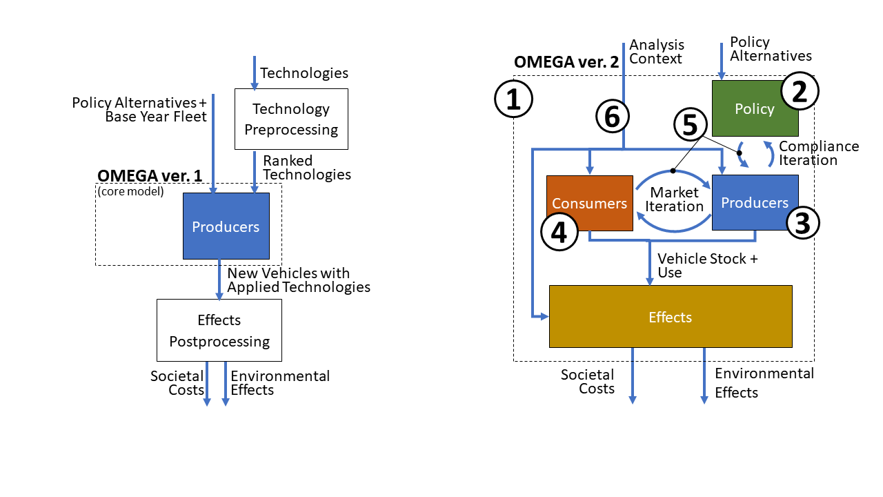
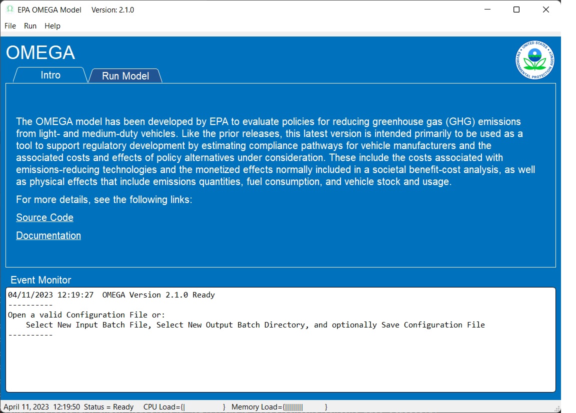
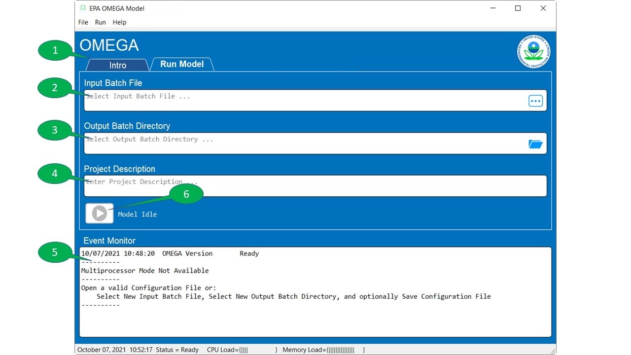
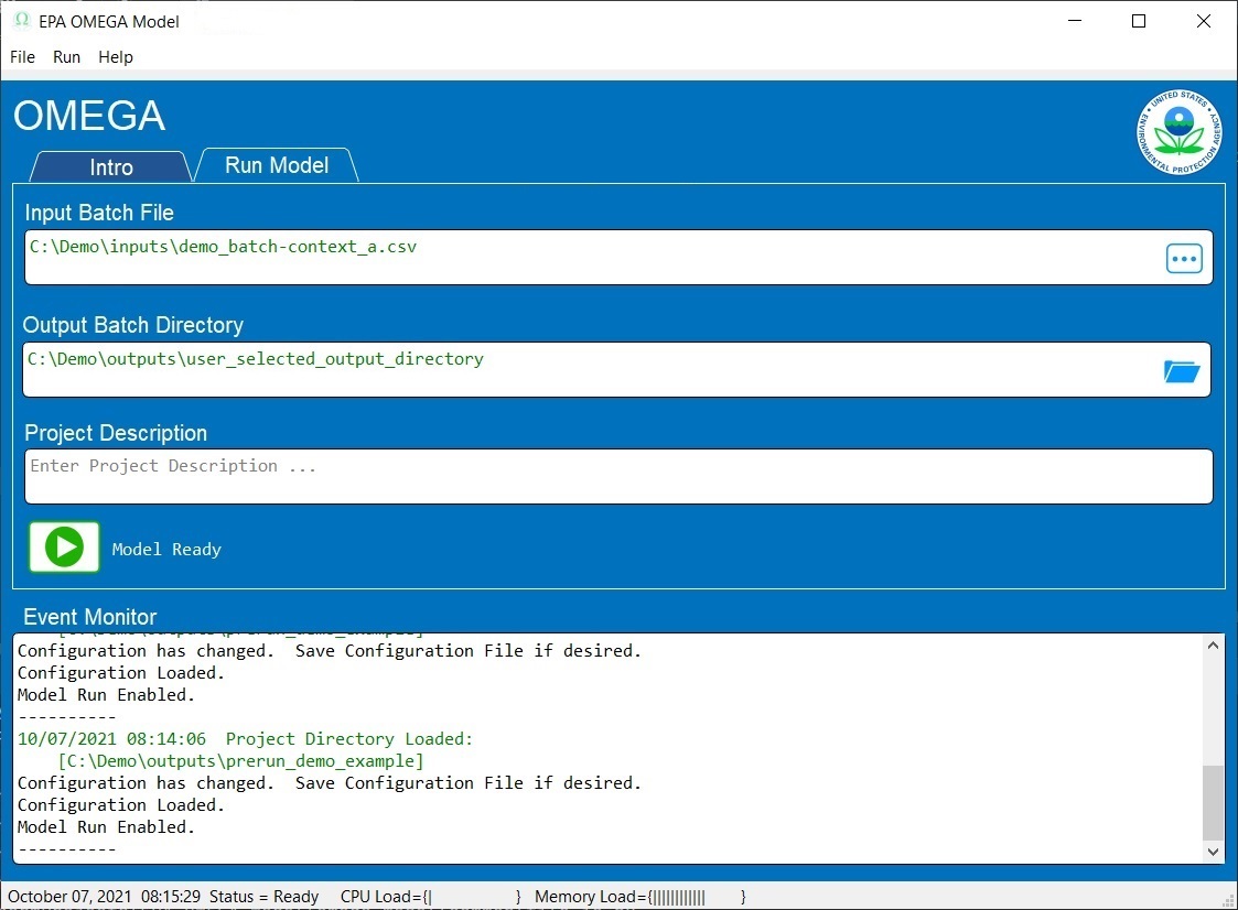
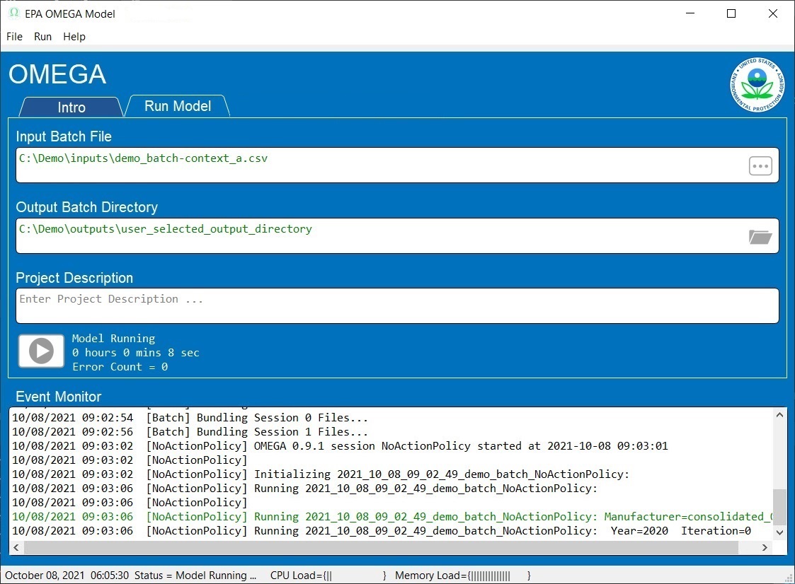
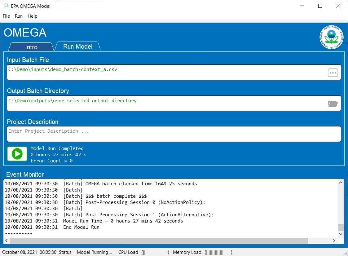
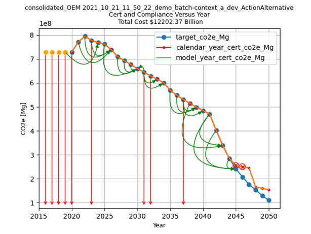
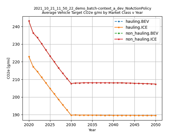
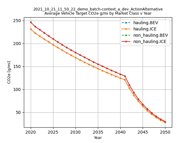
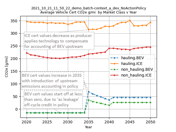
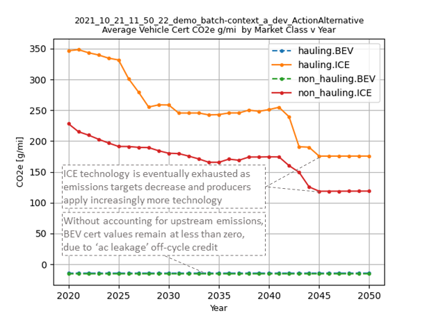

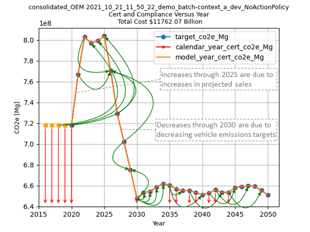
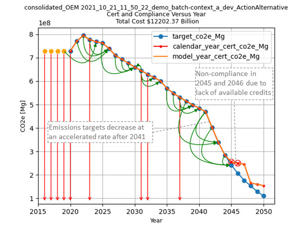
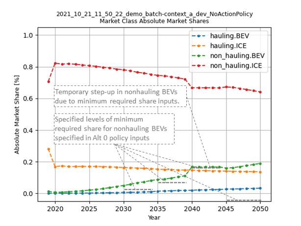
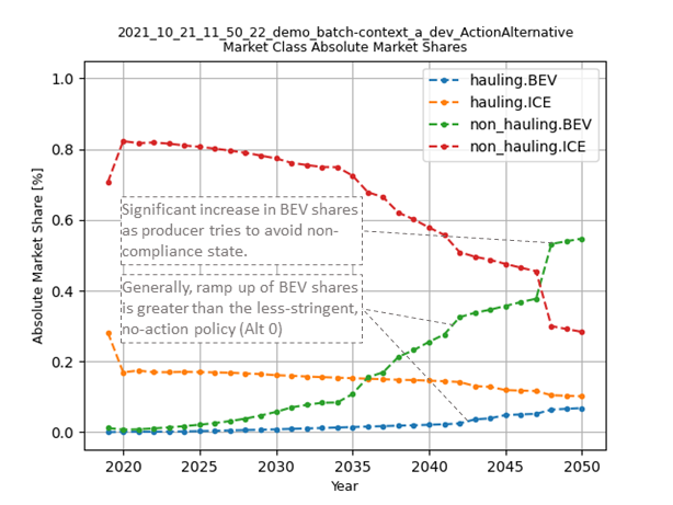
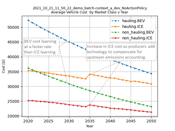
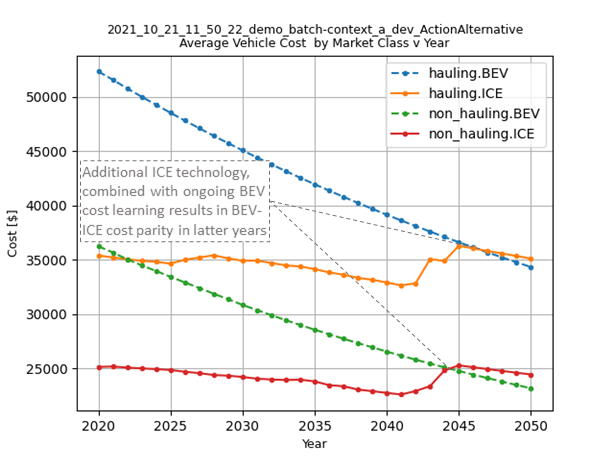
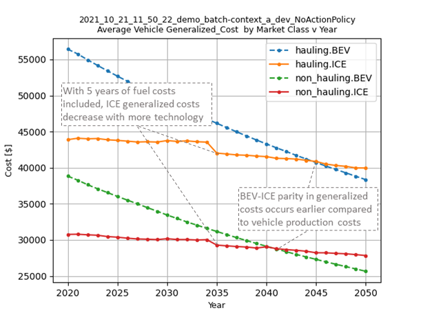
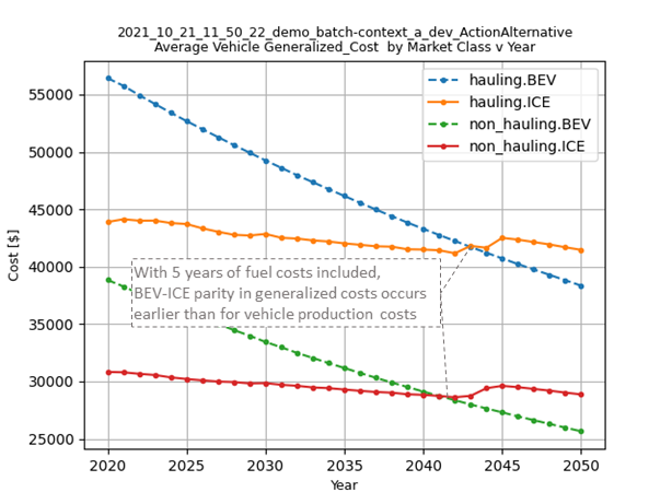
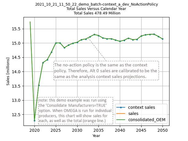
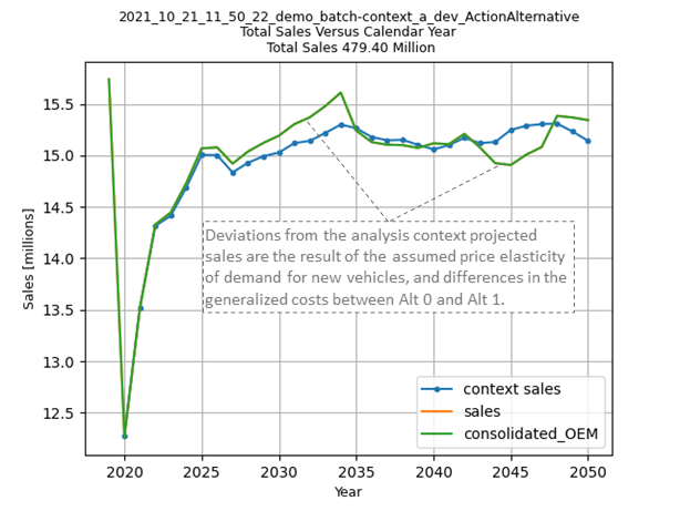
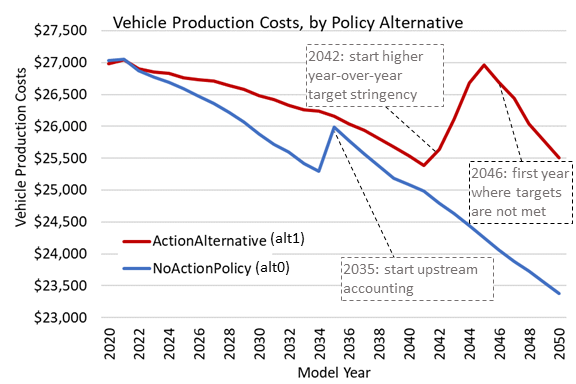
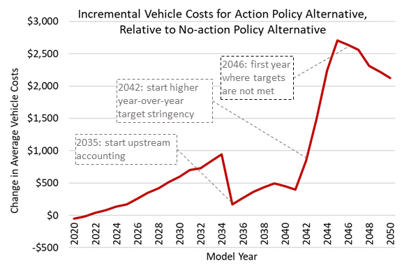
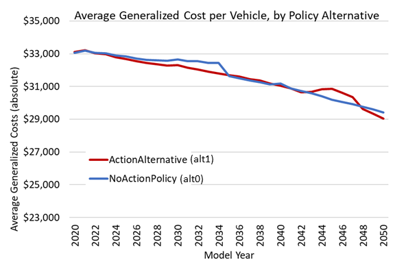
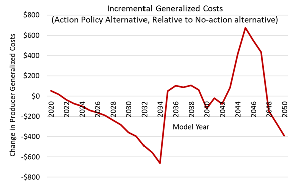
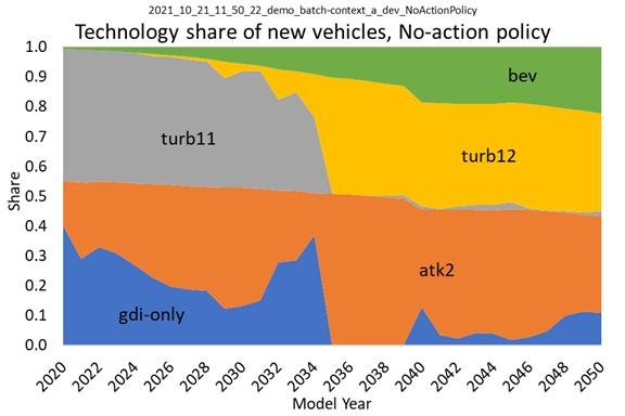
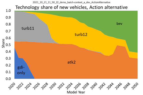
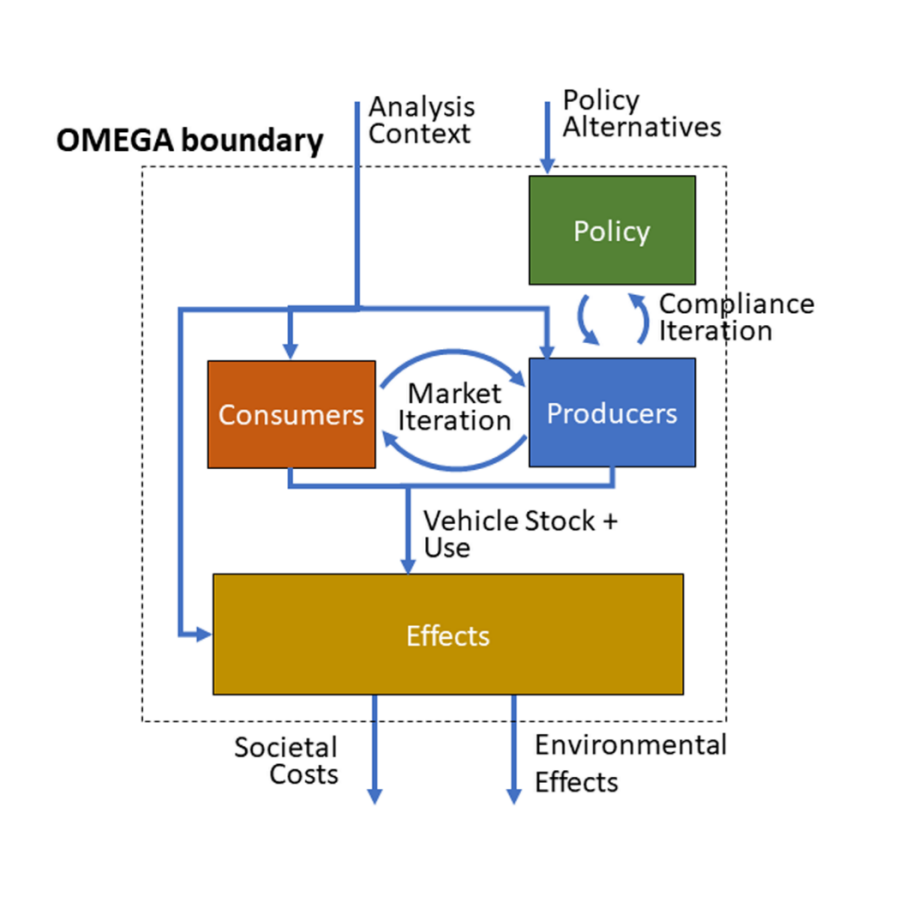
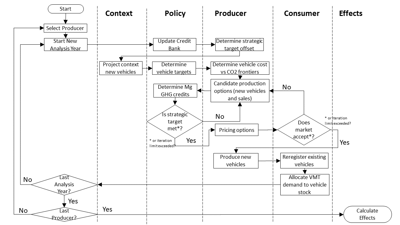
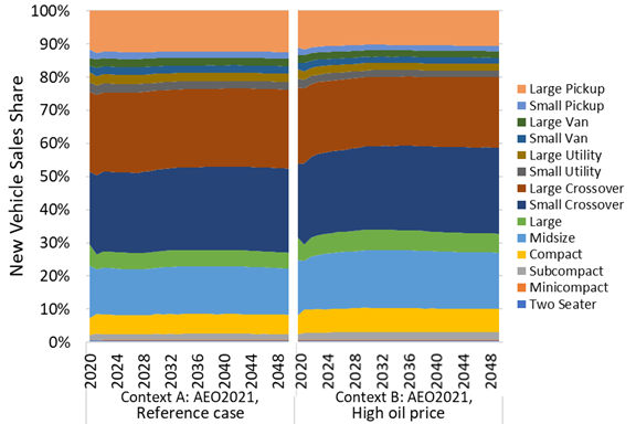
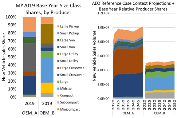
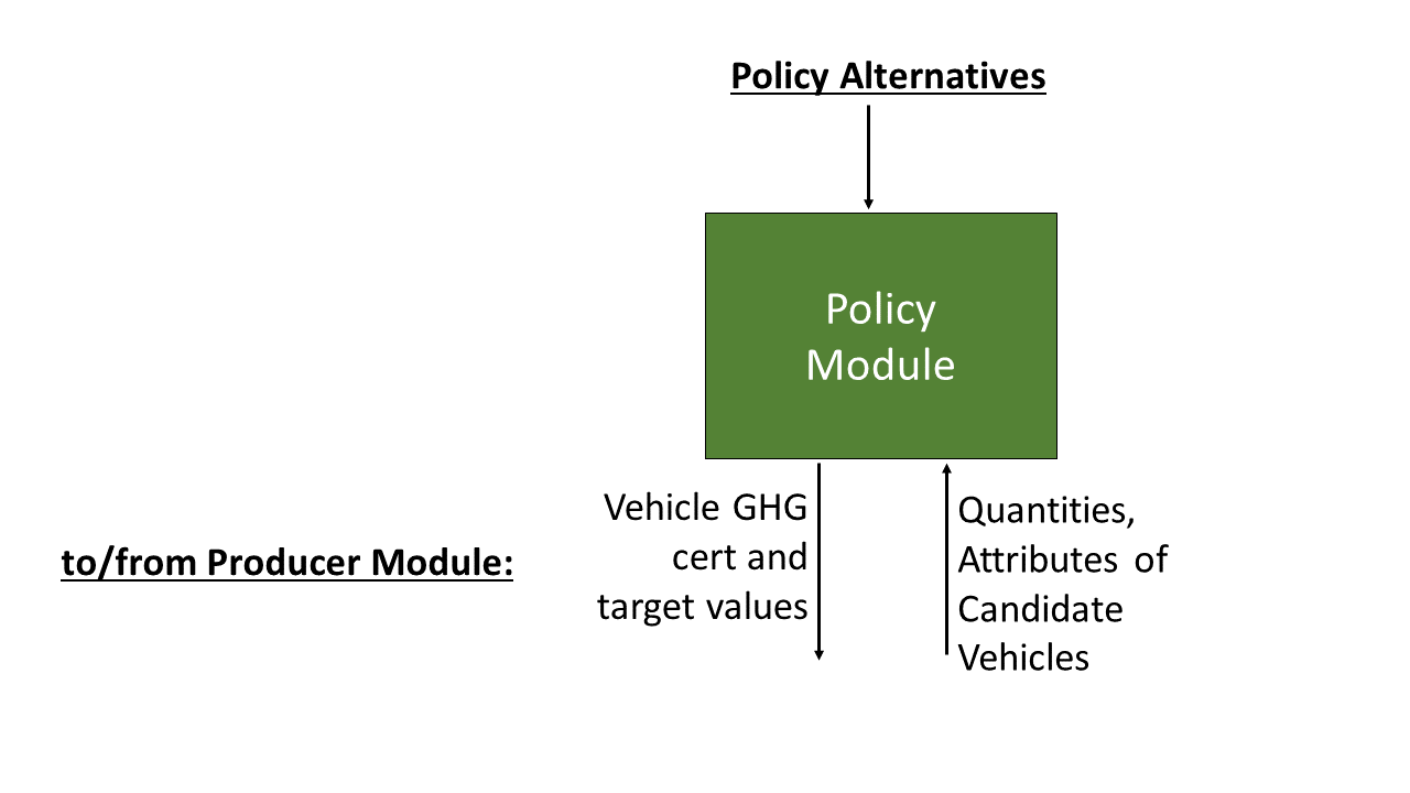
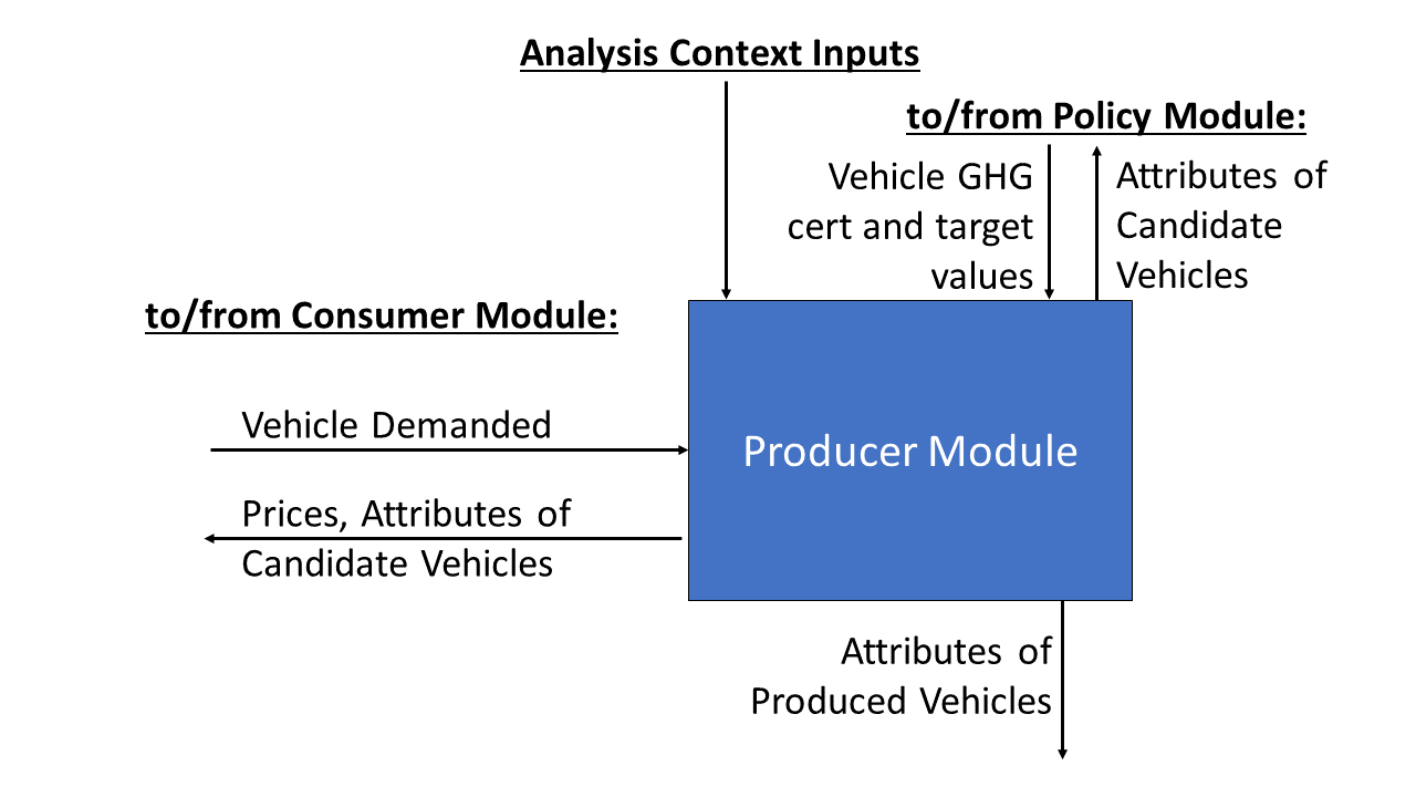
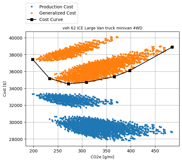
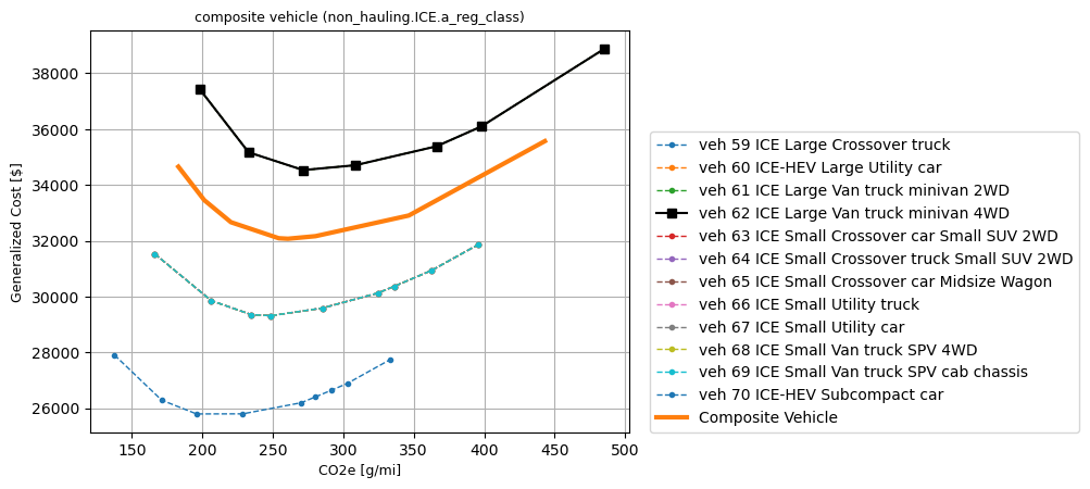
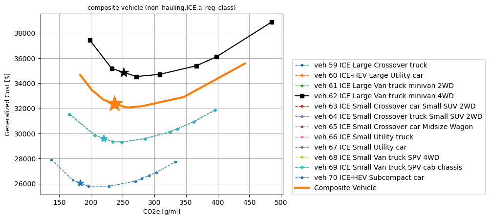
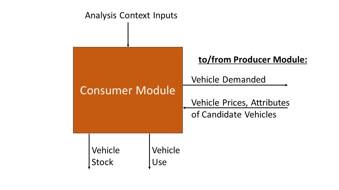
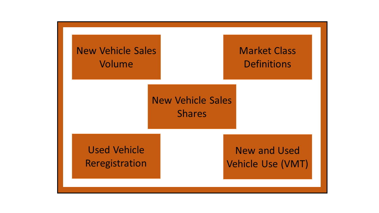
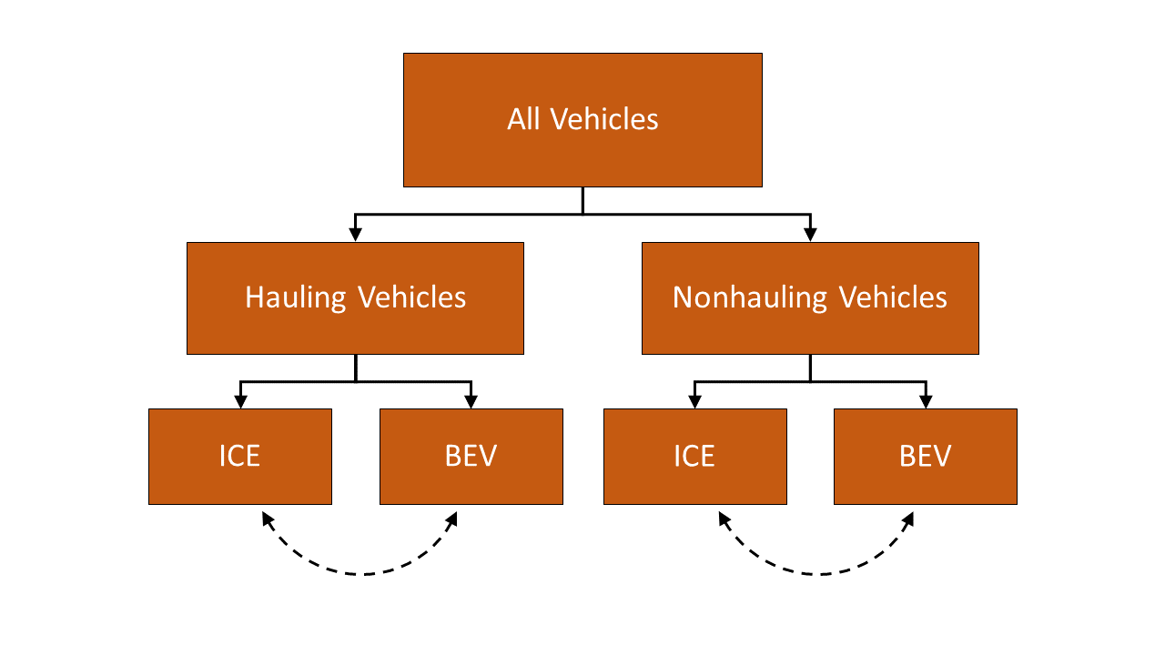

 is the elasticity of demand
 is the change in the quantity demanded
 is the quantity demanded before the price changes
 is the change in the good’s price
 is the good’s price before the change
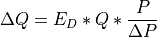
is the share of vehicles in market class i
is the share weight of market class i. This determines how quickly consumers accept new technology.
is the generalized cost of each vehicle in market class i
represents how sensitive the model is to price.
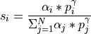
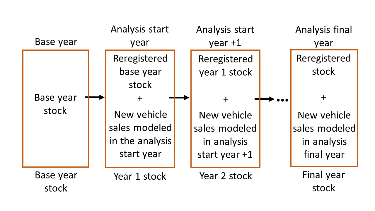
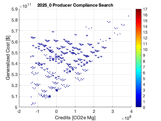
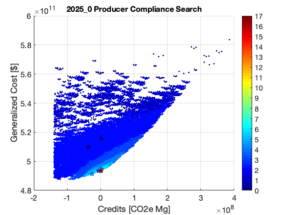
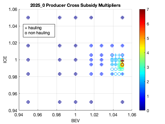
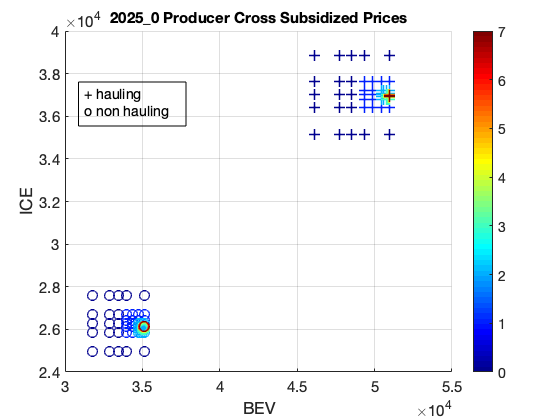
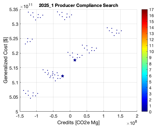
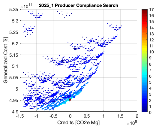
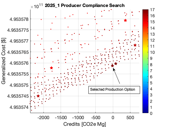
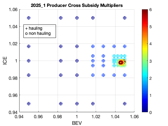
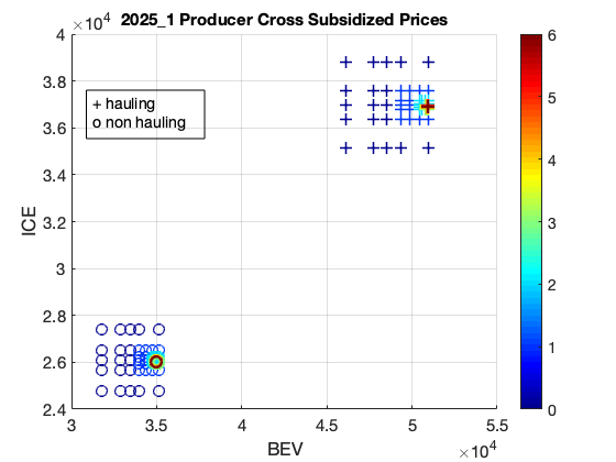
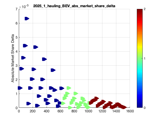
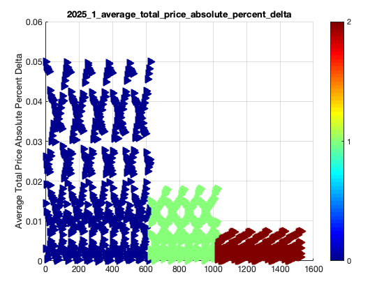
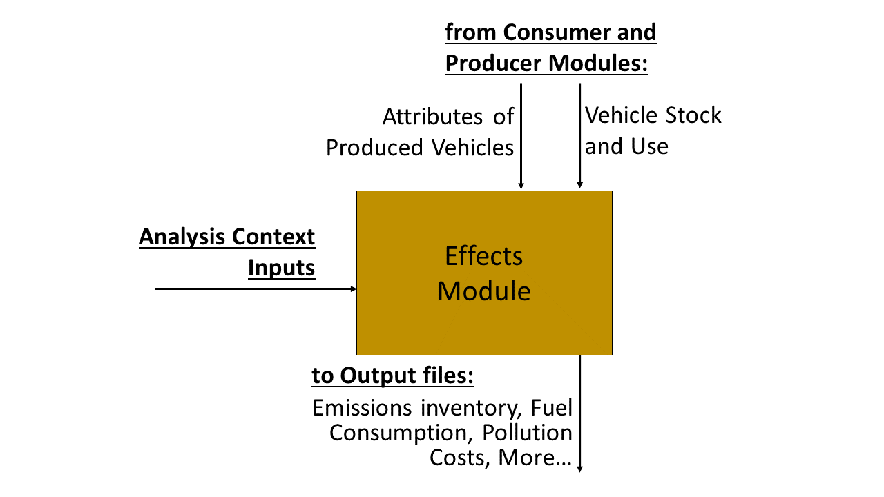


 is calculated within OMEGA and accounts for any credits that do not improve fuel consumption and test-to-onroad gaps
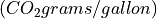 is the
  content of the in-use, or retail, fuel
 is calculated within OMEGA and accounts for any credits that do not improve fuel consumption and test-to-onroad gaps
 is the efficiency of the energy transfer from the charge point to the battery as set by the user
 would be any of the criteria air pollutants such as VOC, PM2.5, NOx, etc., with the exception of
 (which is calculated interanlly in OMEGA)
 is an emission rate from the vehicle emission rates input file
 = 907,185
 is calculated by equation (4.4)
 is the
 or
or 
 = 1,000,000


 is the
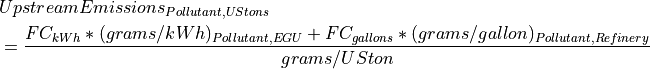
 is
is  calculated by equation (4.5)
 is the Electricity Generating Unit (or Power Sector) emission factor for the given Pollutant
 is
is  calculated by equation (4.4)
 is the Refinery emission rate for the given pollutant
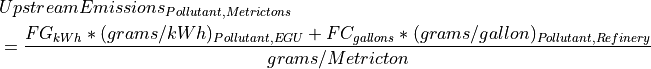
 is
is 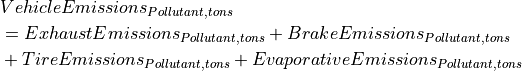
 is calculated by the applicable exhaust emission equation
 is calculated by (4.10)
 is calculated by (4.11)
 is calculated by (4.12)
 is calculated by equation
  is calculated by equation
 is calculated by equation
  is calculated by equation